We use cookies and other tracking technologies to improve your browsing experience on our website, to show you personalized content and targeted ads, to analyze our website traffic, and to understand where our visitors are coming from.
⚠️
GDPR & Cookie Policy Notice
In accordance with data protection regulations; the use of mandatory cookies is required for the core functions of our website to operate, ensure data security, and perform analytics. If you reject the use of cookies, it is not possible to benefit from the services on our website due to technical limitations and data synchronization interruptions. You must consent to the use of cookies to access the content on our site.
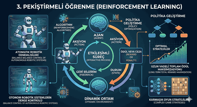
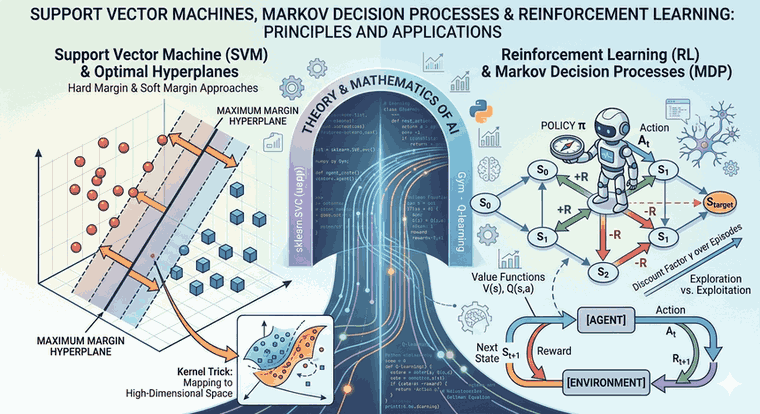
Reinforcement Learning: Dynamic Decision Mechanisms and the Mathematics of Autonomous Systems
Reinforcement Learning (RL) is a discipline in the machine learning hierarchy that is sharply distinguished from supervised and unsupervised learning, based on the “trial-and-error” mechanism in behavioral psychology. Rather than recognizing patterns in static datasets, RL optimizes the sequence of actions an agent takes in an uncertain environment to maximize cumulative reward.
Figure 1: Reinforcement Learning: Dynamic Decision Mechanisms and the Mathematics of Autonomous Systems.
RL Fundamentals and Markov Decision Processes (MDP)
The mathematical skeleton of reinforcement learning is formed by Markov Decision Processes (MDP). An RL problem is generally defined by a quintuple $(S, A, P, R, \gamma)$:
S (State Space): The set of all possible states the agent can be in.
A (Action Space): All actions the agent can perform in a state.
P (Transition Probability): The probability of transitioning to state $s'$ when taking action $a$ in state $s$, denoted as $P(s' | s, a)$.
R (Reward Function): The immediate feedback received after a transition, $R(s, a, s')$.
$\gamma$ (Discount Factor): The coefficient determining the present value of future rewards ($0 \le \gamma \le 1$).
The agent’s primary goal is to develop a Policy ($\pi$) that dictates which action is best for every state. In this process, Value Functions ($V$) and Action-Value Functions ($Q$) are used to estimate the agent’s long-term success.
Policy Optimization and Gradient Methods
In the RL world, solutions generally fall into two main branches: Value-based and Policy-based methods. Policy optimization aims to model the agent’s behavior directly through a set of parameters ($\theta$).
The core logic here is to find the values of $\theta$ that maximize the expected total reward $J(\theta)$. Policy Gradient algorithms update parameters by calculating the gradient of this function:
This approach yields much more stable results in continuous action spaces (e.g., the precise angle of a robotic arm) compared to traditional Q-Learning methods.
Deep Reinforcement Learning (Deep RL) and Architectural Structures
Traditional RL methods encounter the “curse of dimensionality” when the state space grows. In modern systems, this is overcome by using Convolutional Neural Networks (CNN) or Recurrent Neural Networks (RNN) as function approximators.
Deep Q-Networks (DQN)
DQN combines the classic Q-Learning algorithm with deep neural networks. It uses two critical techniques to ensure training stability:
Experience Replay: The agent stores its past experiences in a memory pool and trains by sampling randomly.
Target Network: The network used to calculate target Q-values is updated at regular intervals.
Actor-Critic Models
This hybrid architecture features two different structures:
Actor: Updates the policy (decides which action to take).
Critic: Estimates the value of the taken action (evaluates the action).
Modern algorithms such as PPO (Proximal Policy Optimization) and SAC (Soft Actor-Critic) have become the standard in autonomous driving and robotic balance control by using this structure.
Software Ecosystem and Implementation Libraries
Libraries that have become industry standards for developing RL projects include:
OpenAI Gymnasium: Standard API for environment interfaces.
Stable Baselines3: Reliable RL algorithm implementations based on PyTorch.
Ray Rllib: Production-level tools for scalable, distributed RL training.
Technical Implementation: A Basic Q-Learning Algorithm (Python)
Below is the raw Python implementation of a Q-Learning mechanism that enables an agent to find the optimal route in a simple environment (GridWorld):
import numpy as np
import random
classQLearningAgent:
def__init__(self, states_n, actions_n, lr=0.1, gamma=0.95, epsilon=0.1):
# Initialization of the Q-table (State x Action) self.q_table = np.zeros((states_n, actions_n))
self.lr = lr # Learning rate (Alpha) self.gamma = gamma # Discount factor self.epsilon = epsilon # Exploration ratedefchoose_action(self, state):
# Epsilon-greedy strategyif random.uniform(0, 1) < self.epsilon:
return random.randint(0, self.q_table.shape[1] -1) # Explorationelse:
return np.argmax(self.q_table[state]) # Exploitationdeflearn(self, state, action, reward, next_state):
# Updating the Q-value according to the Bellman Equation old_value = self.q_table[state, action]
next_max = np.max(self.q_table[next_state])
# Q(s,a) = (1-alpha)*Q(s,a) + alpha*(R + gamma * max Q(s',a')) new_value = (1- self.lr) * old_value + self.lr * (reward + self.gamma * next_max)
self.q_table[state, action] = new_value
# Example usage scenario (Pseudo-Environment)states_count =16# 4x4 Gridactions_count =4# Up, Down, Right, Leftagent = QLearningAgent(states_count, actions_count)
# Training Loop (Episode Loop)for episode in range(1000):
state =0# Starting point done =Falsewhilenot done:
action = agent.choose_action(state)
# Responses from the environment (Simulated) next_state = random.randint(0, 15)
reward =1if next_state ==15else-0.1 done =Trueif next_state ==15elseFalse agent.learn(state, action, reward, next_state)
state = next_state
Balance Control and Robotics in Autonomous Systems
Reinforcement learning plays a critical role in high-degree-of-freedom (DoF) systems where classical control theory (such as PID or LQR) is insufficient.
Inverted Pendulum: The RL agent learns to keep the system balanced by adjusting torque values through continuous data streams.
Bipedal Walking: The relationship between joint angles, ground friction, and center of gravity of the robot is optimized with millions of simulation steps (massively parallel simulation).
Important Note: The “Sim-to-Real” problem is the biggest obstacle in transferring RL models to real physical hardware. Domain Randomization techniques are used to bridge the gap between perfect physics in simulation and sensor noise in the real world.
Advanced Concepts: Exploration vs. Exploitation Dilemma
One of the greatest challenges of RL is the balance between whether the agent should follow the best path it knows (Exploitation) or try new things in the hope of finding a better path (Exploration).
Upper Confidence Bound (UCB): Incorporates uncertainty into the reward function to encourage the agent to visit less-frequented states.
Entropy Regularization: An entropy term is added to the cost function to prevent the policy from collapsing into a single action at too early a stage.
The Dynamic Nature of Data Flow
In static deep learning, the dataset is fixed and training iterates over this data. In RL, however, Data is Generated by the Agent’s Own Policy. If the agent follows a poor policy, the data it collects will also be of poor quality. This “positive feedback loop” makes the training of RL systems quite sensitive and sometimes unstable. Therefore, hyperparameter optimization (learning rate, discount factor, batch size) is the key to success in RL projects.
Conclusion and Future Projection
Reinforcement learning is transforming artificial intelligence from being merely a “prediction tool” into a “decision-making” actor. The successes we see today in game strategies (AlphaGo, Dota 2 OpenAI Five) will form the basis for the management of energy grids, high-frequency financial transactions, and autonomous surgical robots tomorrow. As technical depth increases, issues such as sample efficiency and safe RL will remain the focus of research.