We use cookies and other tracking technologies to improve your browsing experience on our website, to show you personalized content and targeted ads, to analyze our website traffic, and to understand where our visitors are coming from.
⚠️
GDPR & Cookie Policy Notice
In accordance with data protection regulations; the use of mandatory cookies is required for the core functions of our website to operate, ensure data security, and perform analytics. If you reject the use of cookies, it is not possible to benefit from the services on our website due to technical limitations and data synchronization interruptions. You must consent to the use of cookies to access the content on our site.
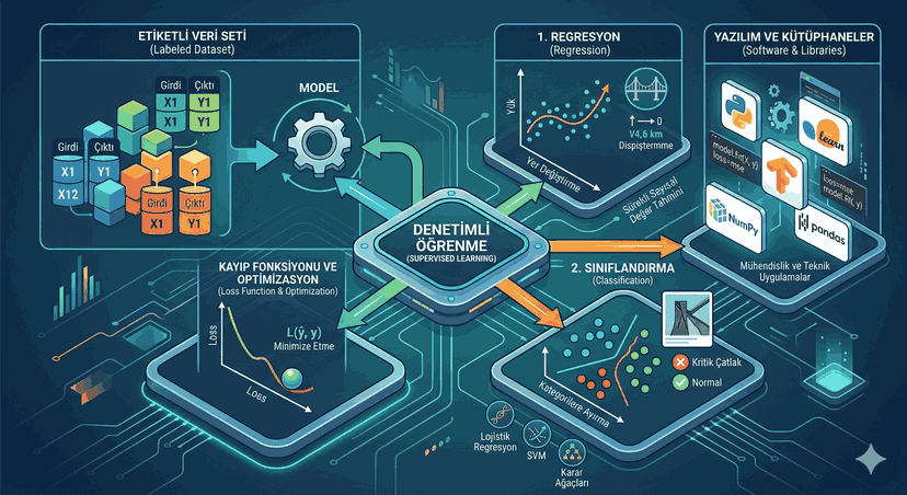
Mathematical Optimization and Applied Algorithm Strategies in Supervised Learning Architecture
Supervised Learning, the cornerstone of the artificial intelligence and machine learning universe, is essentially a function approximation problem. The system utilizes structured datasets to learn the underlying relationship between input vectors ($x$) and target labels ($y$). In this process, the fundamental goal is to capture patterns in the training data to ensure that the model can make generalizations with the lowest possible error rate on data it has never encountered before.
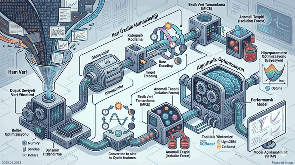
Figure 1: Mathematical Optimization and Applied Algorithm Strategies in Supervised Learning Architecture.
1. Mathematical Foundations and Loss Functions
At the heart of supervised learning lie Loss Functions, which quantify the difference between the model’s predictions and the actual values. Optimization algorithms update model parameters (weights and biases) to minimize the value of this function.
Mean Squared Error (MSE): The most commonly used metric in regression problems. It penalizes large deviations more heavily by squaring the errors.
Cross-Entropy (Log Loss): In classification problems, it measures the difference between the predicted probability distribution and the actual distribution. It is particularly used in deep learning models along with sigmoid or softmax activations.
Note: To prevent the model from “memorizing” the training data (overfitting), L1 (Lasso) or L2 (Ridge) regularization techniques should be incorporated into the loss function.
Regression is a critical discipline for predicting numerical and continuous data. It is used in a wide range of fields, from engineering calculations to financial modeling.
Advanced Approaches:
Multiple Linear Regression: Measures the effect of multiple independent variables on the dependent variable.
Polynomial Regression: Increases complexity by adding high-degree terms in cases where the relationship between data is non-linear and curvilinear.
Random Forest Regression: Reduces variance and provides more stable results by running decision trees in an ensemble manner.
Example Application: Regression Model with Python and Scikit-Learn
The code block below demonstrates a basic pipeline structure that performs regression analysis on a structural dataset:
import numpy as np
import pandas as pd
from sklearn.model_selection import train_test_split
from sklearn.preprocessing import StandardScaler
from sklearn.ensemble import RandomForestRegressor
from sklearn.metrics import mean_squared_error, r2_score
# Creating a synthetic dataset (e.g., Load and Displacement)data = {
'load_kn': np.random.rand(100) *1000,
'material_elasticity': np.random.rand(100) *200,
'displacement_mm': np.random.rand(100) *50}
df = pd.DataFrame(data)
# Preparing the dataX = df[['load_kn', 'material_elasticity']]
y = df['displacement_mm']
X_train, X_test, y_train, y_test = train_test_split(X, y, test_size=0.2, random_state=42)
# Feature Scalingscaler = StandardScaler()
X_train_scaled = scaler.fit_transform(X_train)
X_test_scaled = scaler.transform(X_test)
# Training the modelmodel = RandomForestRegressor(n_estimators=100, max_depth=10, random_state=42)
model.fit(X_train_scaled, y_train)
# Prediction and Evaluationpredictions = model.predict(X_test_scaled)
print(f"MSE: {mean_squared_error(y_test, predictions)}")
print(f"R2 Score: {r2_score(y_test, predictions)}")
3. Classification and Decision Boundaries
Classification is the process of assigning data to predefined discrete categories. In this process, the algorithm tries to find the optimal Decision Boundary that separates the classes from each other.
Fundamental Algorithms and Mechanisms:
Logistic Regression: Although named regression, it is actually a classification algorithm. It uses the logistic (sigmoid) function to compress outputs into a probability value between 0 and 1.
Support Vector Machines (SVM): Finds the hyperplane that maximizes the margin (gap) between classes. With the “Kernel Trick” method, it can classify non-linear data by projecting it into high-dimensional spaces.
XGBoost / LightGBM: These gradient boosting-based libraries combine weak learners to exhibit some of the strongest classification performance available today.
Note: In imbalanced datasets, looking only at the accuracy rate can be misleading. In such cases, analysis should be performed using Precision, Recall, and F1-Score metrics.
4. Image Processing and Deep Supervised Learning
The most advanced stage of supervised learning is image classification and object detection using Convolutional Neural Networks (CNNs). Images are processed as pixel matrices, and the model automatically learns features such as edges, corners, or textures in a hierarchical structure.
Layer Architecture:
Convolutional Layer: Creates feature maps through filters.
Pooling: Reduces dimensionality to decrease computational load and increases the model’s spatial tolerance to features.
Fully Connected Layer: Connects the learned features to class labels.
Example Application: Binary Classification with TensorFlow/Keras
A simple architecture used to classify cracks in a structural element as “critical” or “normal”:
import tensorflow as tf
from tensorflow.keras import layers, models
defcreate_model():
model = models.Sequential([
# First convolutional layer layers.Conv2D(32, (3, 3), activation='relu', input_shape=(128, 128, 3)),
layers.MaxPooling2D((2, 2)),
# Second convolutional layer layers.Conv2D(64, (3, 3), activation='relu'),
layers.MaxPooling2D((2, 2)),
# Flattening and Dense layers layers.Flatten(),
layers.Dense(64, activation='relu'),
layers.Dropout(0.5), # To prevent overfitting layers.Dense(1, activation='sigmoid') # Binary classification output ])
model.compile(optimizer='adam',
loss='binary_crossentropy',
metrics=['accuracy'])
return model
crack_detector = create_model()
crack_detector.summary()
5. Software Ecosystem and Library Selection
In modern AI projects, efficiency depends on selecting the right tools. Libraries that have become industry standards include:
Scikit-Learn: The primary choice for traditional machine learning algorithms (SVM, Decision Trees, Regression) and data preprocessing tools.
PyTorch / TensorFlow: Powerful frameworks that offer GPU support for deep learning, neural networks, and large-scale tensor calculations.
OpenCV: Essential for image preprocessing, filtering, and data preparation in computer vision projects.
Pandas & NumPy: Provide the foundational infrastructure for vector calculations, data manipulation, and matrix operations.
Matplotlib & Seaborn: Used for visualizing data distribution, correlation matrices, and model performance metrics.
6. Data Preparation and Feature Engineering
The success of a supervised learning model is directly related to the quality of the data it is fed. From an engineering perspective, data preparation steps should include:
Imputation: Filling missing values with the mean, median, or regression predictions.
Categorical Encoding: Converting textual classes (e.g., “Damaged”, “Intact”) into numerical values (One-Hot Encoding or Label Encoding).
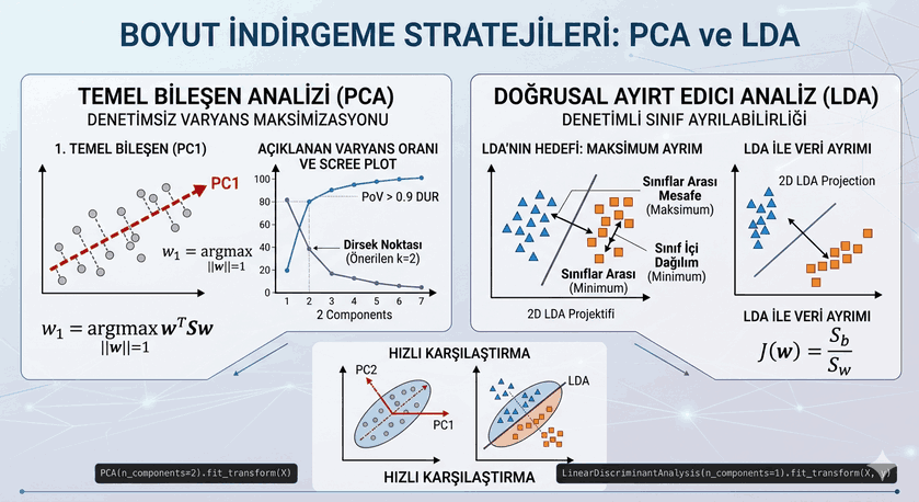
Dimensionality Reduction (PCA): Applying principal component analysis to reduce model complexity and escape the effects of the “curse of dimensionality.”
7. Hyperparameter Optimization
The default settings of algorithms do not always yield the best results. To push model performance to its peak, hyperparameters should be optimized using Grid Search or Randomized Search methods. For example, in an SVM model, fine-tuning the C parameter (error tolerance) and gamma (decision boundary curvature) directly affects the model’s success.
Final Note: The supervised learning process is not a linear path, but a cycle. Steps such as data collection, modeling, testing, and error analysis should be repeated until target metrics are achieved. Especially in technical projects, it is not enough for the model to simply show high success; it must also be explainable (explainable AI), which is of great importance for understanding the parametric reasons behind the decisions made.