We use cookies and other tracking technologies to improve your browsing experience on our website, to show you personalized content and targeted ads, to analyze our website traffic, and to understand where our visitors are coming from.
⚠️
GDPR & Cookie Policy Notice
In accordance with data protection regulations; the use of mandatory cookies is required for the core functions of our website to operate, ensure data security, and perform analytics. If you reject the use of cookies, it is not possible to benefit from the services on our website due to technical limitations and data synchronization interruptions. You must consent to the use of cookies to access the content on our site.
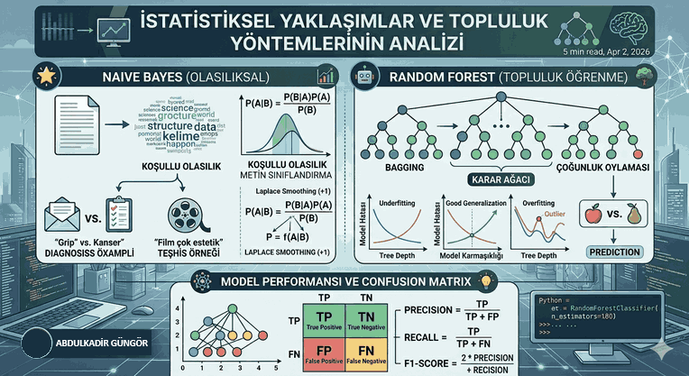
Engineering Analysis of Statistical Approaches and Ensemble Methods in Machine Learning
The artificial intelligence ecosystem is shaped by algorithms based on different mathematical foundations in the process of extracting meaning from data. Although Deep Learning is popular in modern software architectures, classical machine learning algorithms still form the backbone of the industry in terms of computational cost and explainability.
Figure 1: Engineering Analysis of Statistical Approaches and Ensemble Methods in Machine Learning.
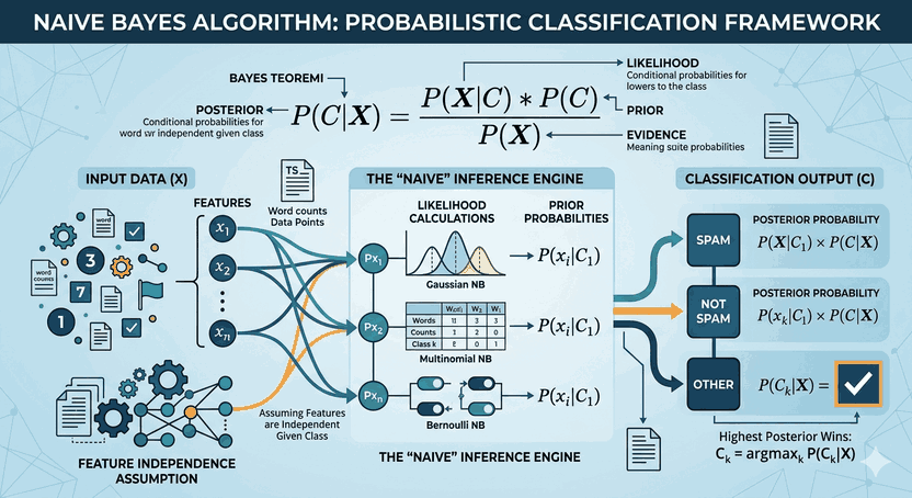
1. The Mathematical Foundation of Naive Bayes and Probabilistic Classification
Naive Bayes is an algorithm based on Thomas Bayes’ probability theory that shows high performance, especially in high-dimensional textual data (NLP). The term “Naive” in the algorithm’s name comes from the assumption that features are completely independent of each other. From an engineering perspective, although this assumption does not always hold true in real life (for example, words in a sentence are dependent on each other), it incredibly increases the computational speed of the algorithm.
Bayes’ Theorem and Conditional Probability
Bayes’ theorem converts the probability of an event occurring into an updated probability (posterior) based on prior knowledge (prior) regarding that event:
$$P(A|B) = \frac{P(B|A) \cdot P(A)}{P(B)}$$
Where:
$P(A|B)$: The probability of A occurring when event B occurs (Posterior).
$P(B|A)$: The probability of observing B given that event A is true (Likelihood).
$P(A)$: The initial probability of A (Prior).
$P(B)$: The total probability of the evidence (Evidence).
Laplace Smoothing and the Zero Probability Problem
In text analysis, when a word that has never been seen in the training set appears in the test set, it reduces the chain of probabilities in multiplication to zero. To overcome this problem, the Laplace Smoothing method is used. By adding $+1$ to each frequency, the generalization ability of the model is preserved.
Python Implementation (Scikit-Learn):
from sklearn.feature_extraction.text import CountVectorizer
from sklearn.naive_bayes import MultinomialNB
from sklearn.pipeline import Pipeline
# Creating a model pipeline for text datatext_clf = Pipeline([
('vect', CountVectorizer()), # Word frequency vector ('clf', MultinomialNB(alpha=1.0)) # NB with Laplace smoothing (alpha)])
corpus = ["The film is very aesthetic and impressive", "A waste of time production"]
labels = [1, 0] # 1: Positive, 0: Negativetext_clf.fit(corpus, labels)
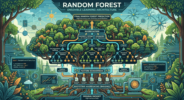
2. Transition from Decision Trees to Random Forest Architecture
Decision trees are hierarchical structures that split data into branches based on specific threshold values. However, a single decision tree is prone to overfitting the training data. This is where Random Forest comes in, an ensemble algorithm using the “Bagging” (Bootstrap Aggregating) technique.
Entropy and Information Gain in Decision Trees
Information Gain or Gini Impurity determines how a node is split. Mathematically, entropy ($H$) represents the uncertainty in a system:
$$H(S) = -\sum_{i=1}^{c} p_i \log_2(p_i)$$
Random Forest selects random samples from the dataset and creates thousands of different trees using random feature subsets for each tree. The result is determined by the voting (classification) or averaging (regression) of these trees.
Overfitting and Pruning Strategies
If the tree depth ($max\_depth$) is not limited, the model starts to learn the noise.
Pre-pruning: Stopping the tree at a certain depth or minimum sample count while it is being formed.
Post-pruning: Cutting off branches that do not increase the error rate after the tree is completed.
3. Advanced Ensemble Methods: Gradient Boosting
While Random Forest trees are trained in parallel and independently, Gradient Boosting (GBM) follows a sequential path. Each new tree is constructed to minimize the residual errors made by the previous tree.
Libraries such as XGBoost, LightGBM, and CatBoost, which are frequently preferred in engineering applications, are optimized versions of this logic. Especially in structured (tabular) data, these models often outperform deep learning models.
4. Model Performance Analysis and Confusion Matrix
Evaluating a model’s success solely through “Accuracy” is a major mistake, especially in imbalanced datasets. For example, if only 5 out of 1000 people in a group are ill, the model saying everyone is “healthy” gives 99.5% accuracy, but it is medically unsuccessful because it cannot detect any patients.
Precision: How many of the positive predictions are truly correct. Important if the cost of a false alarm (FP) is high.
$$Precision = \frac{TP}{TP + FP}$$
Recall (Sensitivity): How many of the actual positives are captured. Critical if the cost of missing a case (FN) is high (such as cancer diagnosis).
$$Recall = \frac{TP}{TP + FN}$$
F1-Score: The harmonic mean of Precision and Recall. It is the most reliable metric in cases of class imbalance.
5. Application Architecture and Code Example
The block below contains a comprehensive Python example involving the training of a Random Forest model and the analysis of its performance with detailed metrics.
import numpy as np
import pandas as pd
from sklearn.model_selection import train_test_split
from sklearn.ensemble import RandomForestClassifier
from sklearn.metrics import confusion_matrix, classification_report, f1_score
# Creating a synthetic datasetfrom sklearn.datasets import make_classification
X, y = make_classification(n_samples=1000, n_features=20, n_classes=2, weights=[0.9, 0.1], random_state=42)
# Train and test splitX_train, X_test, y_train, y_test = train_test_split(X, y, test_size=0.2, random_state=42)
# Hyperparameter configuration of the Random Forest modelmodel = RandomForestClassifier(
n_estimators=100,
max_depth=10,
min_samples_split=5,
class_weight='balanced', # Weighting for imbalanced datasets random_state=42)
model.fit(X_train, y_train)
y_pred = model.predict(X_test)
# Model evaluationprint("Confusion Matrix:\n", confusion_matrix(y_test, y_pred))
print("\nDetailed Report:\n", classification_report(y_test, y_pred))
6. Engineering Notes and Architectural Decision Making
In machine learning projects, model selection varies according to the structure of the data and business requirements:
If Data Amount is Small: Low-variance models like Naive Bayes can be preferred.
If Data Dimensionality is High (NLP): A combination of TF-IDF or Word2Vec vectors with Multinomial Naive Bayes provides a balance of speed/performance.
If Interpretability is Required: Decision trees or logistic regression are ideal for visualizing why the model made a decision.
If Maximum Performance is Required: Random Forest or Gradient Boosting models optimized with hyperparameters (using GridSearchCV or Optuna) should be used.
Notes on Hardware and Memory Management
When working with large datasets, memory management (RAM) becomes critical. The Random Forest algorithm can use all CPU cores in parallel with the n_jobs=-1 parameter. However, if the tree depth increases uncontrollably, the space occupied by the model (pickle file size) can reach gigabyte levels. This should be kept in mind when deploying models, especially in embedded systems or on servers with limited resources (Edge Computing).
Conclusion and Evaluation
Machine learning is not just about choosing an algorithm; it is the art of understanding the statistical distribution of the data and matching the most appropriate mathematical model to that distribution. Naive Bayes’ probability-based approach, Random Forest’s ensemble power, and Confusion Matrix’s analytical depth form the cornerstones of a robust artificial intelligence system. Although advanced Transformer models have revolutionized large-scale problems, the engineering discipline always requires choosing the tool that “solves the problem most efficiently,” not the “most complex one.”