We use cookies and other tracking technologies to improve your browsing experience on our website, to show you personalized content and targeted ads, to analyze our website traffic, and to understand where our visitors are coming from.
⚠️
GDPR & Cookie Policy Notice
In accordance with data protection regulations; the use of mandatory cookies is required for the core functions of our website to operate, ensure data security, and perform analytics. If you reject the use of cookies, it is not possible to benefit from the services on our website due to technical limitations and data synchronization interruptions. You must consent to the use of cookies to access the content on our site.
Theoretical Foundations and Application Strategies of the Naive Bayes Algorithm
In the world of machine learning, probabilistic approaches offer a robust and computationally efficient foundation, especially for classification problems. Naive Bayes is a “generative” modeling approach based on Bayes’ Theorem and the assumption of independence between variables. Its high performance, even on complex datasets, makes it an indispensable tool in fields such as natural language processing (NLP) and spam detection.
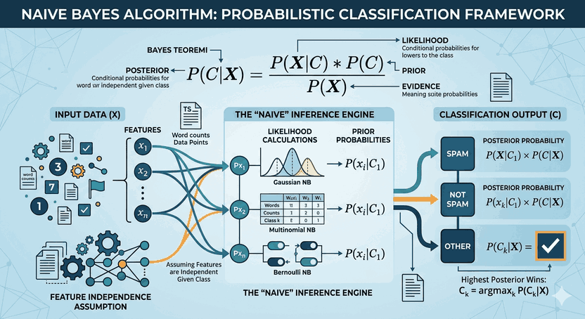
Figure 1: Theoretical Foundations and Application Strategies of the Naive Bayes Algorithm.
Probabilistic Framework and Bayes’ Theorem
Naive Bayes calculates the probability of a data point belonging to a specific class based on the conditional probabilities of the features belonging to that class. Bayes’ Theorem is expressed with the following formula:
$$P(C|X) = \frac{P(X|C) \cdot P(C)}{P(X)}$$
Where:
$P(C|X)$: The probability of class $C$ occurring given data $X$ (Posterior).
$P(X|C)$: The probability of observing data point $X$ given that class $C$ is known (Likelihood).
$P(C)$: The frequency of class $C$ in the total data (Prior).
$P(X)$: The general distribution probability of the data (Evidence).
The point that makes the Naive Bayes model “naive” is the assumption that all features are independent of each other. In other words, the occurrence of a word in an email does not affect the probability of other words occurring. Mathematically:
Depending on the structure of the data, different Naive Bayes variants are used:
1. Gaussian Naive Bayes
It is preferred in cases where features have continuous values and show a normal (Gaussian) distribution. The probability density function is calculated using the mean ($\mu$) and variance ($\sigma^2$) of each feature:
It is used in frequency-based data such as text classification. Features are represented by the number of times an event occurs (e.g., word count).
3. Bernoulli Naive Bayes
It is used in cases where features are only binary (boolean) (e.g., does the word exist in the text or not?).
Practical Application and Python Libraries
In the Python ecosystem, scikit-learn is the most optimized library for Naive Bayes applications. Below is a basic structure for using MultinomialNB on text data.
from sklearn.feature_extraction.text import CountVectorizer
from sklearn.naive_bayes import MultinomialNB
from sklearn.pipeline import make_pipeline
# Example datasetdata = ["spam advertising content", "business meeting report", "you won the sweepstakes"]
labels = [1, 0, 1]
# Pipeline setup: Vectorization + Modelmodel = make_pipeline(CountVectorizer(), MultinomialNB())
# Trainingmodel.fit(data, labels)
# Predictionprint(model.predict(["business meeting"]))
Advantages and Limitations
Naive Bayes works quite fast on large datasets. The training process can be completed in a single pass of the data ($O(n \cdot d)$ complexity). However, the “independence assumption” is often violated in real-world data. While the meaning of a word depends on the word preceding it, Naive Bayes ignores this context.
Note: If one of the features in the data has never been seen in the training set, the probability multiplication will be zero. To prevent this, the Laplace Smoothing technique is used. This technique eliminates the zero probability problem by adding a small value to all probabilities.
Advanced Optimizations
To increase the success of the model, the following strategies should be applied:
Feature Selection: Cleaning unnecessary features (noise) increases the accuracy of the model.
Log-Space Calculation: When probability values are very small, multiplication leads to an “underflow” error in computers. Therefore, logarithmic summation is preferred:
Balanced Dataset: Naive Bayes can be sensitive to minority classes. The dataset should be balanced using sampling methods (oversampling/undersampling).
Conclusion
Naive Bayes is a building block of machine learning architectures with its simplicity and mathematical elegance. Although it is not as complex as deep learning models (Transformer, BERT, etc.), it continues to be one of the best models in resource-constrained systems and situations requiring rapid prototyping, with the correct hyperparameter optimizations.