We use cookies and other tracking technologies to improve your browsing experience on our website, to show you personalized content and targeted ads, to analyze our website traffic, and to understand where our visitors are coming from.
⚠️
GDPR & Cookie Policy Notice
In accordance with data protection regulations; the use of mandatory cookies is required for the core functions of our website to operate, ensure data security, and perform analytics. If you reject the use of cookies, it is not possible to benefit from the services on our website due to technical limitations and data synchronization interruptions. You must consent to the use of cookies to access the content on our site.
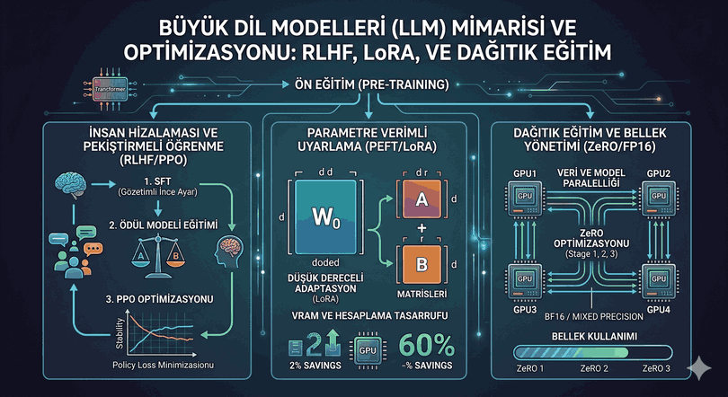
Architectural Depth of Large Language Models: Alignment, Optimization, and Efficient Adaptation
As the artificial intelligence ecosystem evolves from raw transformer blocks to assistant models interacting with users, a massive engineering operation takes place in the background. A Large Language Model (LLM) is more than just billions of parameters; how these parameters are aligned, optimized under hardware constraints, and adapted for specific tasks are the fundamental factors determining a model’s success.
Figure 1: Architectural Depth of Large Language Models: Alignment, Optimization, and Efficient Adaptation.
1. Post-Training Alignment: RLHF and the PPO Mechanism
During the pre-training stage, the model learns language and the world by performing “Next Token Prediction.” However, this stage is insufficient for the model to understand user intent or provide safe responses. RLHF (Reinforcement Learning from Human Feedback) is the gold standard used to align the model with human values.
RLHF Pipeline
RLHF consists of three critical stages:
SFT (Supervised Fine-Tuning): The model is trained on high-quality question-answer pairs.
Reward Model (RM) Training: Humans rank different responses (A and B) generated by the model. With this data, a separate RM is trained that scores “how good” a text is.
Reinforcement with PPO (Proximal Policy Optimization): The model is updated to receive high scores from the RM.
The PPO algorithm uses KL Divergence (Kullback-Leibler Divergence) to prevent the model (Policy) from making too radical changes. If the model strays too far from its original weights, a penalty mechanism is triggered.
# PPO Update Logic (Conceptual PyTorch Example)import torch.nn.functional as F
defcompute_ppo_loss(old_log_probs, new_log_probs, advantages, clip_range=0.2):
ratio = torch.exp(new_log_probs - old_log_probs)
surr1 = ratio * advantages
surr2 = torch.clamp(ratio, 1.0- clip_range, 1.0+ clip_range) * advantages
policy_loss =-torch.min(surr1, surr2).mean()
return policy_loss
2. GRPO: Group Relative Policy Optimization
GRPO (Group Relative Policy Optimization), which replaces PPO in modern models (such as DeepSeek-V3), increases efficiency by reducing the need for a separate Reward Model (RM). In GRPO, the model generates a group of outputs ($G$) for the same input. The quality of each output is evaluated relative to other outputs in the group.
Here, $r_i$ is the reward of the i-th output. Instead of an absolute reward score, this method allows the model to choose the one that is “better than the other options in the group.” This offers a much more stable learning curve, especially in deterministic fields like mathematical proving and coding.
3. Parameter-Efficient Fine-Tuning (PEFT) and LoRA
Fully training a model with billions of parameters (e.g., Llama-3 70B) requires massive VRAM. LoRA (Low-Rank Adaptation) freezes the model’s original weights ($W_0$) and expresses the weight change ($\Delta W$) as the product of two low-rank matrices.
Mathematical Formulation:
Instead of updating a $d \times d$ matrix, two matrices ($A$ and $B$) with dimensions $d \times r$ and $r \times d$ are used. Here, $r$ (rank) is usually a very small value, such as 8 or 16.
$$W = W_0 + B \cdot A$$
This technique can reduce the number of parameters to be trained by 10,000%.
QLoRA: 4-Bit Quantization and Double Quantization
QLoRA takes LoRA a step further by compressing the main model into 4-bit in NormalFloat4 (NF4) format. This allows a 65-billion parameter model to be trained on a single 48GB GPU.
In LLM training, the memory (VRAM) bottleneck stems not only from model weights but also from Optimizer States and Gradients. The use of FP32 (Single Precision) is very precise but memory-intensive.
FP16 / BF16: Modern GPUs (A100, H100) support the BFloat16 format. Although BF16 occupies the same memory space as FP16, it has the same dynamic range (exponent) as FP32. This minimizes the risk of “underflow/overflow” during training.
Mixed Precision Training: While calculations are performed in low precision (FP16/BF16), a master copy of the weights is kept in high precision (FP32).
5. Distributed Training and ZeRO Optimization
For models that do not fit on a single GPU, ZeRO (Zero Redundancy Optimizer) protocols developed by DeepSpeed are used:
ZeRO-1: Partitions optimizer states across GPUs.
ZeRO-2: Also partitions gradients to reduce memory load.
ZeRO-3 (Full Parameter Sharding): Also partitions model weights. When a layer is to be processed, the relevant GPU gathers the weights from others, performs the operation, and then deletes them.
6. Knowledge Distillation and Pruning
Transferring the knowledge of large models to small models (Knowledge Distillation) is critical for running LLMs on edge devices.
Soft Targets: The student model mimics not only the most probable word of the teacher model but its entire probability distribution (logits).
Structured Pruning: Structures with low importance (e.g., attention heads or layers) in the model are completely removed. This allows the model to operate in a “sparse” structure.
7. Inference Process and Parallelization Strategies
After the model is trained, the throughput (how many tokens can be generated per second) is critical for commercial success.
Tensor Parallelism (TP): Splits a single matrix multiplication operation across multiple GPUs. Requires very high-speed communication (NVLink).
Pipeline Parallelism (PP): Splits the model on a layer-by-layer basis. GPU 1 processes the first 10 layers, GPU 2 processes the next 10 layers.
Continuous Batching: Fills an empty slot with a new request as soon as a user’s response finishes, preventing the GPU from remaining idle (the basis of the vLLM library).
Technical Note: LLM optimization is an art of “balance.” While a balance between creativity and accuracy is established with KL Divergence; a balance between hardware cost and performance is established with LoRA and Quantization. The models of the future will not be larger, but will possess “smart” optimization layers that process data more effectively.