We use cookies and other tracking technologies to improve your browsing experience on our website, to show you personalized content and targeted ads, to analyze our website traffic, and to understand where our visitors are coming from.
⚠️
GDPR & Cookie Policy Notice
In accordance with data protection regulations; the use of mandatory cookies is required for the core functions of our website to operate, ensure data security, and perform analytics. If you reject the use of cookies, it is not possible to benefit from the services on our website due to technical limitations and data synchronization interruptions. You must consent to the use of cookies to access the content on our site.
The Anatomy of Modern Deep Learning: A Technical Journey from Gradients to Attention Mechanisms
The revolution in the world of artificial intelligence over the last decade is essentially the result of the perfect synchronization of mathematical optimization, linear algebra, and hardware capabilities. Deep learning is not just about multi-layer neural networks; it is an engineering art that has fundamentally changed how we represent data.
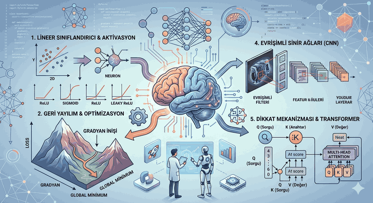
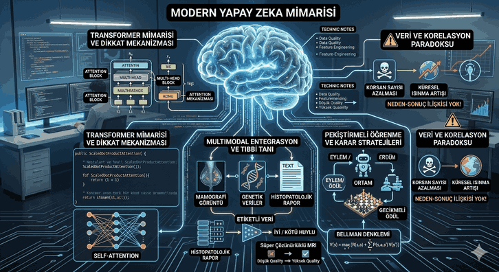
Figure 1: The Anatomy of Modern Deep Learning: A Technical Journey from Gradients to Attention Mechanisms
1. Transition from Linear Classification to Multi-Layer Structures
Everything starts with a simple linear equation where we obtain a score by multiplying input vectors with weight matrices. Expressed mathematically, the score for an input vector $x$ is calculated as $f(x, W) = Wx + b$. Here, $W$ represents the weight matrix, and $b$ represents the bias term.
However, real-world data is rarely linearly separable. Linear models are insufficient even for the most basic logical operations like the XOR problem. At this point, Activation Functions come into play. Activation functions add “non-linearity” to the network, enabling the realization of the Universal Approximation Theorem.
Basic Activation Functions and Code Equivalents
ReLU (Rectified Linear Unit): The most common function with the lowest computational cost. It zeros out negative values and leaves positive values as they are.
Sigmoid: Compresses the output into the $[0, 1]$ range, but can lead to the “vanishing gradient” problem in deep networks.
Leaky ReLU: Adds a small slope ($0.01x$) to solve the “dead neuron” problem of ReLU in the negative region.
2. The Engine of Deep Learning: Backpropagation and Automatic Differentiation
A model’s “learning” is actually the process of finding weight parameters that minimize the prediction error (Loss). This process is managed by Backpropagation, which is based on the Chain Rule.
In the Forward Pass, data flows through the layers and a loss value is calculated. In backpropagation, the partial derivative of this loss with respect to each weight is taken. This derivative creates a “vector field” showing how much each parameter contributed to the error.
Modern libraries (PyTorch, TensorFlow) perform these derivative calculations automatically via a Computational Graph.
3. Optimization Strategies: Faster and More Stable Learning
Although Gradient Descent is a fundamental method, it causes issues such as getting stuck in local minima or progressing excessively slowly with massive datasets. Therefore, various optimization algorithms have been developed.
Major Optimization Techniques
SGD (Stochastic Gradient Descent): Uses a small piece (batch) of data instead of the whole dataset at each step. It is noisy but gains speed.
Momentum: Uses the concept of acceleration in physics to remember the previous direction of the gradient. This reduces “oscillations” and speeds up on flat surfaces.
Adam (Adaptive Moment Estimation): Uses both momentum and the moving average of the squared gradients (RMSProp). It is accepted as the standard today.
# Adam Optimization example in PyTorchimport torch.optim as optim
model = MyNeuralNetwork()
optimizer = optim.Adam(model.parameters(), lr=0.001, betas=(0.9, 0.999))
# Within the training loopoptimizer.zero_grad() # Reset gradientsloss = criterion(output, target)
loss.backward() # Backpropagationoptimizer.step() # Update parameters
4. The Architect of Visual Data: Convolutional Neural Networks (CNN)
CNNs are designed to preserve spatial hierarchy in images. Unlike traditional Fully Connected layers, CNNs learn local features using filters (kernels).
Convolution: The process of sliding a filter over an image to create feature maps.
Pooling: Reduces the dimension of the data (Max Pooling is generally used) and ensures the model is robust against small shifts.
CNNs learn simple geometric shapes like edges and corners in the initial layers, and object parts and complex structures as they go deeper.
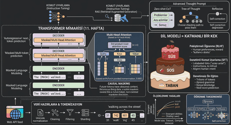
5. The Peak of Modern Artificial Intelligence: Attention and Transformer
The structure that dominates the field of Natural Language Processing (NLP) and now image processing (Vision Transformers) is the Attention mechanism. Unlike RNNs (Recurrent Neural Networks), the Attention mechanism sees the entire input at once and mathematically calculates how much each part relates to the other.
QKV (Query, Key, Value) Logic
The attention process is carried out through three basic vectors:
Query: What the current word is looking for.
Key: What other words offer.
Value: The actual information content.
The attention score is calculated by taking the dot product of the Query and Key vectors and normalized using the Softmax function:
The Transformer architecture performs this process many times in parallel (Multi-Head). In this way, the model can simultaneously learn both grammatical relationships and semantic contexts within the same sentence in different “heads.”
# A basic Self-Attention mechanism (PyTorch style pseudocode)import torch.nn.functional as F
defself_attention(query, key, value):
d_k = query.size(-1)
# Calculate scores scores = torch.matmul(query, key.transpose(-2, -1)) / np.sqrt(d_k)
# Convert to probability distribution weights = F.softmax(scores, dim=-1)
# Multiply with valuesreturn torch.matmul(weights, value)
6. Stabilization and Regularization in Training
Training becomes more difficult as deep networks get deeper. There are two critical techniques used to overcome this:
Batch Normalization: Ensures gradients flow more healthily by normalizing the input of each layer.
Dropout: Prevents the model from memorizing (overfitting) by randomly turning off some neurons during training.
Technical Note:Layer Normalization, used in large language models (LLMs), works independently of the batch size, so it gives more successful results than Batch Norm in sequential data.
7. Hardware and Scalability: The GPU and TPU Factor
Deep learning algorithms are inherently built on matrix multiplications. While a CPU is adept at performing complex logical operations in sequence, it is not designed to perform thousands of small matrix multiplications simultaneously. GPU (Graphics Processing Unit) and the TPU (Tensor Processing Unit) developed by Google have enabled deep learning to reach its current speed by completing these parallel operations in milliseconds with their thousands of cores.
Libraries like CUDA (NVIDIA) and ROCm (AMD) allow developers to perform tensor operations directly on the graphics processor.
Conclusion: Layers of the Future
Deep learning is a point where mathematical elegance, algorithmic efficiency, and massive processing power converge. The error correction journey, which started with backpropagation, has evolved into human-level text and image generation with Transformer models containing billions of parameters today. From an engineering perspective, even the most complex artificial intelligence system is essentially a whole composed of correctly tuned weights, optimized gradients, and carefully selected activation functions.
In the coming period, focus will be placed on these models not only being “larger” but also “more efficient” (inference optimization) and “more explainable” (explainable AI). The heart of deep learning continues to beat in these dynamic algorithms that continue to discover hidden patterns within data.