We use cookies and other tracking technologies to improve your browsing experience on our website, to show you personalized content and targeted ads, to analyze our website traffic, and to understand where our visitors are coming from.
⚠️
GDPR & Cookie Policy Notice
In accordance with data protection regulations; the use of mandatory cookies is required for the core functions of our website to operate, ensure data security, and perform analytics. If you reject the use of cookies, it is not possible to benefit from the services on our website due to technical limitations and data synchronization interruptions. You must consent to the use of cookies to access the content on our site.
The Quest for Balance in Model Optimization: A Stability Analysis of Machine Learning from Underfitting to Overfitting
In the modern world of computing, while the terms automation and artificial intelligence are often used interchangeably, these two disciplines reside in different layers from an engineering perspective. Automation is built upon a deterministic structure; it executes specific tasks within the framework of predefined code blocks and algorithmic rules without requiring external intervention. However, as the complexity of systems has increased, these rigid rules have been replaced by artificial intelligence (AI) systems that learn from data and develop dynamic decision-making mechanisms.
Artificial intelligence does not merely execute instructions; it also simulates human cognitive processes to discover latent correlations within data. At the heart of this discovery process lies Machine Learning, the art of mathematical modeling that transforms data into information and information into predictions.
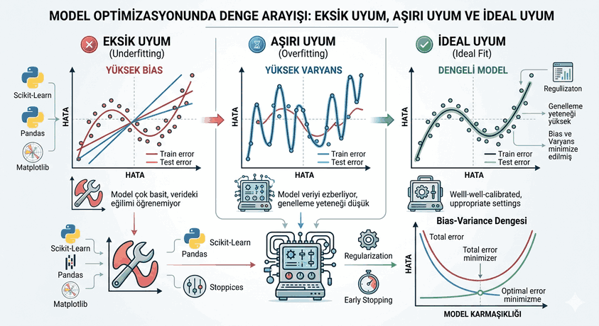
Figure 1: The Quest for Balance in Model Optimization: A Stability Analysis of Machine Learning from Underfitting to Overfitting.
Building Blocks of Machine Learning Architecture
The success of a machine learning system is not a random outcome, but the product of a meticulously crafted data pipeline. Three core components come to the fore in this process:
Data: It is the raw material of the model. However, not every piece of data is “high-quality” data. The data must have high representation power and be as free of noise as possible.
Feature Engineering: It is the selection of meaningful features from input data that will increase the model’s learning capacity. For example, in a housing price prediction model, building age, square footage, and location are critical features.
Model and Algorithm Selection: This is the stage of choosing the appropriate mathematical model based on the type of problem (Classification or Regression).
The Critical Role of Domain Data
The data used during the training of the model must reflect the “real world” conditions in which the model will operate. If you train an autonomous driving algorithm only with data collected in sunny weather, the system will fail at night or in rainy weather. This situation is defined in data science as the domain shift or out-of-distribution data problem.
Model Fit and Error Analysis: Bias and Variance Balance
The greatest challenge in machine learning is maintaining the fine line between the model memorizing the training data and grasping its logic. This balance is known in statistical literature as the Bias-Variance Tradeoff.
1. Underfitting
This occurs when the model is not complex enough to learn the underlying structure in the data. In this case, error rates are high in both training and test data. The model is too simple (high bias).
2. Overfitting
This happens when the model begins to “learn” the noise and random fluctuations in the training data. While it gives perfect results on the training data, it fails on previously unseen test data. The model is overly complex (high variance).
3. Ideal Fit
This is the point where the model captures the general trend, filters out noise, and shows a high ability for generalization to new data.
Technical Implementation: Regression Analysis with Python and Scikit-Learn
Polynomial Regression is one of the best tools to observe a model’s transition from underfitting to overfitting. The code block below uses the scikit-learn library to simulate how models of different complexities fit the data.
import numpy as np
import matplotlib.pyplot as plt
from sklearn.pipeline import Pipeline
from sklearn.preprocessing import PolynomialFeatures
from sklearn.linear_model import LinearRegression
from sklearn.model_selection import cross_val_score
# Creating a synthetic dataset (Noisy sine wave)deftrue_fun(X):
return np.cos(1.5* np.pi * X)
np.random.seed(0)
n_samples =30degrees = [1, 4, 15] # 1: Underfitting, 4: Ideal, 15: OverfittingX = np.sort(np.random.rand(n_samples))
y = true_fun(X) + np.random.randn(n_samples) *0.1plt.figure(figsize=(14, 5))
for i in range(len(degrees)):
ax = plt.subplot(1, len(degrees), i +1)
polynomial_features = PolynomialFeatures(degree=degrees[i], include_bias=False)
linear_regression = LinearRegression()
pipeline = Pipeline([("poly", polynomial_features), ("linear", linear_regression)])
pipeline.fit(X[:, np.newaxis], y)
# Performance evaluation scores = cross_val_score(pipeline, X[:, np.newaxis], y, scoring="neg_mean_squared_error", cv=10)
X_test = np.linspace(0, 1, 100)
plt.plot(X_test, pipeline.predict(X_test[:, np.newaxis]), label="Model")
plt.plot(X_test, true_fun(X_test), label="True Function")
plt.scatter(X, y, edgecolor='b', s=20, label="Data Points")
plt.title(f"Degree {degrees[i]}\nMSE: {-scores.mean():.2e}")
plt.legend(loc="best")
plt.show()
Software Libraries Used to Manage Complexity
A vast ecosystem exists in modern data science projects to optimize models and resolve fitment issues:
Scikit-Learn: The industry standard for general machine learning algorithms, model selection, and preprocessing tools.
TensorFlow & Keras: Used in deep learning models, especially to manage the number of layers (complexity) of neural networks.
Pandas: The fundamental library for the manipulation of structured data and feature engineering processes.
Optuna / Hyperopt: Libraries that automatically determine the “degree” or complexity of a model by performing hyperparameter optimization.
Engineering Notes and Strategic Approaches
To achieve an “ideal fit” during the model development process, the following technical strategies should be followed:
Note 1: Regularization
To prevent overfitting, penalty terms such as L1 (Lasso) or L2 (Ridge) should be used. These techniques trim unnecessary complexity by constraining the model’s coefficients.
Note 2: Early Stopping
In iterative learning processes (e.g., neural networks), training should be halted at the point where the validation error begins to increase. This is one of the most effective methods to prevent the model from memorizing the data.
Note 3: Data Augmentation
If the model is prone to overfitting and more real data cannot be collected, the dataset can be artificially expanded by performing manipulations (rotating, scaling, adding noise) on the existing data.
Note 4: Cross-Validation
Instead of tying the model’s success to a single test set, testing in different combinations by splitting the data into k-folds provides a more reliable metric regarding generalization ability.
Conclusion
Model fit in artificial intelligence systems is not a static goal, but a dynamic balancing process. A data scientist’s duty is not only to achieve the lowest error rate but also to guarantee the performance (robustness) the model will exhibit in new and uncertain environments. The “ideal fit” obtained by avoiding the simplicity of underfitting and the illusion of overfitting transforms artificial intelligence from mere software into an intelligent mechanism that generates solutions in the real world.