We use cookies and other tracking technologies to improve your browsing experience on our website, to show you personalized content and targeted ads, to analyze our website traffic, and to understand where our visitors are coming from.
⚠️
GDPR & Cookie Policy Notice
In accordance with data protection regulations; the use of mandatory cookies is required for the core functions of our website to operate, ensure data security, and perform analytics. If you reject the use of cookies, it is not possible to benefit from the services on our website due to technical limitations and data synchronization interruptions. You must consent to the use of cookies to access the content on our site.
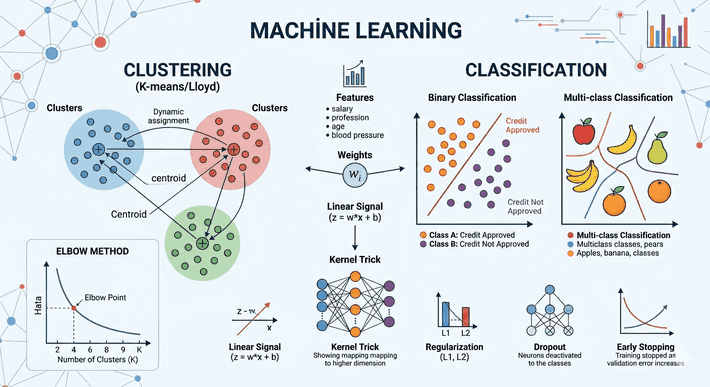
Modern Clustering and Classification Strategies in Machine Learning
In the artificial intelligence and data science ecosystem, the process of transforming raw data into meaningful insights is built upon two fundamental pillars: Supervised and Unsupervised learning. This article will cover everything from linear classification models to the mathematical depth of clustering algorithms, the resolution of overfitting problems via regularization techniques, and practical Python implementations.
Figure 1: Modern Clustering and Classification Strategies in Machine Learning.
Mathematics of Linear Classification and Decision Boundaries
Classification is the process of taking a feature vector ($x$) of a data point as input and mapping it to a predefined discrete label ($y$). In linear classification, the most fundamental approach, the model creates a “decision hyperplane.”
Linear Signal and Activation
The heart of a linear model is the linear signal, which is the weighted sum of input features. Mathematically, it is expressed as:
$$z = \sum_{i=1}^{n} w_i x_i + b$$
Here, the $w$ parameters determine the influence (degree of importance) of each feature on the decision, while the $b$ (bias) term allows the decision boundary to be shifted from the origin. If the dataset is “linearly separable,” algorithms such as the Perceptron Learning Algorithm (PLA) update these weights until a perfect separation is achieved. However, real-world data is rarely this clean. For noisy or slightly overlapped data, the Pocket Algorithm comes into play; this algorithm keeps the best set of weights obtained during the training process in its “pocket.”
Non-Linear Transformations
If the dataset has a circular or complex structure, linear models fail directly. At this point, it is necessary to move the data to a higher-dimensional space using the Kernel Trick or feature engineering. For example, data that cannot be separated on a two-dimensional plane can become separable by a plane when moved to a third dimension using transformations such as $x^2 + y^2$.
Unsupervised Learning and Clustering Architecture
Unlike classification, clustering is used to discover hidden structures when data is not labeled. The main goal is to maximize intra-cluster similarity while minimizing inter-cluster similarity.
Lloyd’s Algorithm and the K-Means Mechanism
K-Means is an iterative displacement algorithm and is often used synonymously with Lloyd’s Algorithm. The algorithm attempts to solve the following optimization problem:
Here, $\mu_j$ is the centroid of the $j$-th cluster. The process works as follows:
Assignment Step: Each data point is assigned to the nearest center (Euclidean distance is used).
Update Step: The centers of the clusters are recalculated by taking the arithmetic mean of all points assigned to that cluster.
K-Means Implementation with Python
The following code block performs and visualizes clustering on a synthetic dataset using the scikit-learn library:
import numpy as np
import matplotlib.pyplot as plt
from sklearn.cluster import KMeans
from sklearn.datasets import make_blobs
# Creating a synthetic datasetX, y = make_blobs(n_samples=500, centers=4, cluster_std=0.60, random_state=0)
# Training the K-Means modelkmeans = KMeans(n_clusters=4, init='k-means++', max_iter=300, n_init=10)
y_kmeans = kmeans.fit_predict(X)
# Visualizationplt.scatter(X[:, 0], X[:, 1], c=y_kmeans, s=50, cmap='viridis')
centers = kmeans.cluster_centers_
plt.scatter(centers[:, 0], centers[:, 1], c='red', s=200, alpha=0.75, marker='X')
plt.title("K-Means Clustering Results")
plt.show()
Model Optimization and Hyperparameter Selection
The most critical question in a clustering model is “How many clusters (K) should there be?” Two basic metrics are used for this:
Elbow Method: The total squared error (Inertia) corresponding to the K value is plotted. The point where the rate of decrease in error suddenly drops and the graph takes the shape of an elbow represents the optimal K value.
Silhouette Score: Measures how similar a point is to its own cluster compared to neighboring clusters, with a value between -1 and +1. Values close to +1 indicate perfect clustering.
Model Flexibility and Regularization Techniques
High-capacity models (complex neural networks or deep decision trees) tend to learn the noise in the training data. This is called Overfitting. Regularization is applied to restrain the model and improve its generalization ability.
Explicit Regularization
In this method, a penalty term is added to the model’s loss function:
L1 (Lasso): Adds the absolute value of the weights. Performs feature selection by pulling some weights exactly to zero.
L2 (Ridge): Adds the square of the weights. Shrinks the weights but does not zero them out, which ensures the coefficients are distributed more evenly.
Implicit Regularization
Instead of directly interfering with the mathematical function, it changes the nature of the training process:
Dropout: Randomly deactivates a certain percentage of neurons during training to prevent the network from becoming dependent on specific paths.
Early Stopping: Stops training as soon as the validation error starts to increase.
Data Augmentation: Increases the data by rotating, scaling, or adding noise, allowing the model to see more variations.
Technical Notes and Implementation Strategies
Feature Scaling: Since K-Means is a distance-based algorithm, data on different scales, such as salary (thousands) and age (tens), must be normalized with StandardScaler or MinMaxScaler. Otherwise, features with large values will dominate the cluster.
Dimensionality Reduction: If there are more than 100 features, PCA (Principal Component Analysis) should be applied before clustering to both reduce noise and lower computational cost.
Algorithm Selection: If the dataset has an elongated form rather than being circular, Gaussian Mixture Models (GMM) or density-based DBSCAN should be preferred over K-Means.
Machine learning models are not just about loading data and getting outputs; this process is a battle of every parameter (weights, bias, K number) with the geometry of the data. Correct regularization and model selection are the keys to an artificial intelligence architecture that wins this battle.