We use cookies and other tracking technologies to improve your browsing experience on our website, to show you personalized content and targeted ads, to analyze our website traffic, and to understand where our visitors are coming from.
⚠️
GDPR & Cookie Policy Notice
In accordance with data protection regulations; the use of mandatory cookies is required for the core functions of our website to operate, ensure data security, and perform analytics. If you reject the use of cookies, it is not possible to benefit from the services on our website due to technical limitations and data synchronization interruptions. You must consent to the use of cookies to access the content on our site.
Advanced Analytical Modeling and Algorithmic Visualization Strategies in High-Dimensional Data Spaces
In the modern data science ecosystem, the process of refining raw data into strategic insights requires the integration of advanced statistical methods, linear algebra operations, and sophisticated software architectures. Data analytics is not just a descriptive process; it is also a computational optimization problem.
Figure 1: Advanced Analytical Modeling and Algorithmic Visualization Strategies in High-Dimensional Data Spaces.
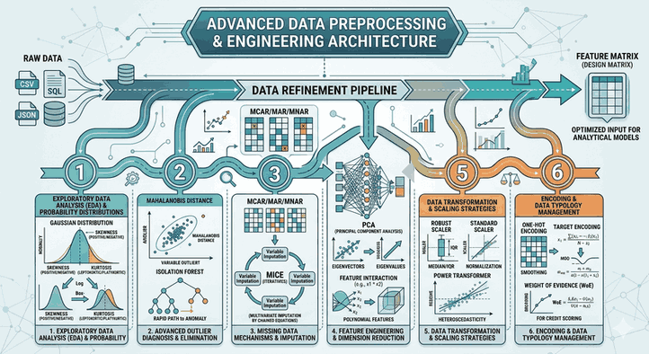
1. Data Preprocessing and Engineering: Algorithmic Approaches
The quality of the dataset is the most fundamental element determining the success of the model. Models built on noisy data are doomed to fail based on the “garbage in, garbage out” principle.
Advanced Imputation: Instead of simple mean assignments, iterative imputer algorithms like MICE (Multivariate Imputation by Chained Equations), which preserve the variance between variables, should be used.
Feature Scaling:StandardScaler (z-score normalization) is mandatory for Gradient Descent-based algorithms (LR, SVM, Neural Networks), while MinMaxScaler is necessary for distance-based algorithms (KNN, K-Means).
import pandas as pd
import numpy as np
from sklearn.experimental import enable_iterative_imputer
from sklearn.impute import IterativeImputer
from sklearn.preprocessing import StandardScaler
# Technical Data Preparation Processdeftechnical_preprocessing(df):
# Missing value management with Iterative Imputation it_imputer = IterativeImputer(max_iter=10, random_state=42)
df_imputed = it_imputer.fit_transform(df)
# Z-Score Normalization scaler = StandardScaler()
df_scaled = scaler.fit_transform(df_imputed)
return pd.DataFrame(df_scaled, columns=df.columns)
2. Statistical Validity and Hypothesis Testing
To prove that the analytical output is not random, parametric and non-parametric tests must be applied. The suitability of the data for normal distribution (Gaussian) should be checked with the Shapiro-Wilk test, and the homogeneity of variances with the Levene test.
Multicollinearity Analysis: High correlation between independent variables makes coefficient estimates unstable. This should be checked by calculating the Variance Inflation Factor (VIF). Variables with a VIF value above 5 should be eliminated from the model.
3. Spectral Analysis and Stationarity in Time Series
In time-oriented data, it should be questioned whether the series is stationary before modeling. If there is a trend or seasonality in the series, unit root tests are applied.
ADF (Augmented Dickey-Fuller) Test: It is the fundamental statistical test that measures the stationarity of the series.
Seasonal Decomposition: Analyzing the data by separating it into trend, seasonality, and residual components optimizes the signal-to-noise ratio (SNR).
from statsmodels.tsa.stattools import adfuller
from statsmodels.tsa.seasonal import seasonal_decompose
deftime_series_validation(series):
# Augmented Dickey-Fuller Test result = adfuller(series)
print(f'ADF Statistic: {result[0]}')
print(f'p-value: {result[1]}')
# Seasonal Decomposition (Additive Model) decomp = seasonal_decompose(series, model='additive', period=12)
return decomp
4. Dimensionality Reduction and Manifold Learning
Visualization is impossible in high-dimensional datasets containing thousands of features. At this point, dimensionality reduction techniques come into play:
PCA (Principal Component Analysis): Creates new orthogonal axes that maximize the variance of the data. It provides a linear transformation via eigenvalues and eigenvectors.
t-SNE and UMAP: Performs non-linear dimensionality reduction by preserving local relationships between data. It is standard for visualizing clustering analysis results in 2D/3D space.
5. Software Architecture and Library Selection
For a high-performance analysis process, integrating the following libraries and tools is critical:
Data Manipulation:Pandas and NumPy (Uses C-based backend for vectorial calculations).
Visualization:
Matplotlib: Low-level, fully controllable charts.
Seaborn: Statistical visualization layer based on Matplotlib.
Deep Learning:PyTorch or TensorFlow (Tensor operations and GPU acceleration).
6. Advanced Techniques in Data Visualization
The “Data-Ink Ratio” principle should be applied in the visual presentation of data. Unnecessary visual clutter (chartjunk) should be eliminated to increase the density of information.
Heatmaps: Used to analyze correlations in feature matrices or confusion matrices.
Parallel Coordinates: Ideal for showing patterns and class separations in multi-dimensional data on a single graph.
Data analytics and visualization are the intersection point of mathematical rigor and software engineering. Successful analysis is a whole discipline extending from understanding the statistical distribution of data to choosing the right dimensionality reduction algorithms and visualizing results in a way that minimizes cognitive load. The correct application of these techniques enables the uncovering of hidden patterns in complex data structures.