We use cookies and other tracking technologies to improve your browsing experience on our website, to show you personalized content and targeted ads, to analyze our website traffic, and to understand where our visitors are coming from.
⚠️
GDPR & Cookie Policy Notice
In accordance with data protection regulations; the use of mandatory cookies is required for the core functions of our website to operate, ensure data security, and perform analytics. If you reject the use of cookies, it is not possible to benefit from the services on our website due to technical limitations and data synchronization interruptions. You must consent to the use of cookies to access the content on our site.
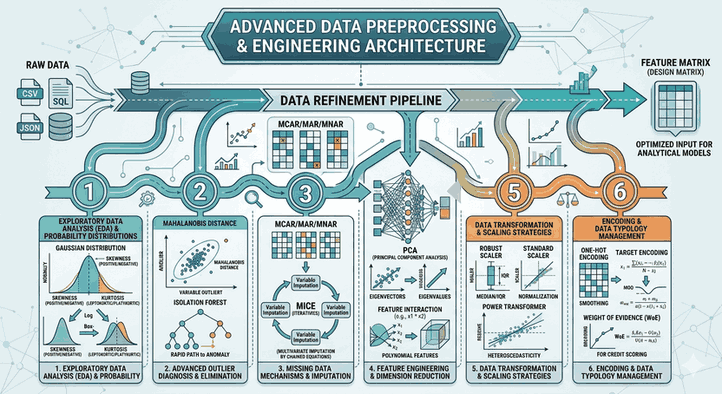
Advanced Data Preprocessing and Engineering Architecture in Data Science
The transformation of data from its raw form into a processed feature matrix in analytical modeling processes is a synthesis of statistical methodologies and computational techniques. In a data mining pipeline, understanding the topological structure of the data and cleansing it of noise directly determines the generalization capability of the final model.
Figure 1: The data refining pipeline extending from the data collection stage to the production of the feature matrix and optimized input.
1. Exploratory Data Analysis (EDA) and Probability Distributions
The initial intervention in the dataset begins with the examination of the probability density functions (PDF) of the variables. A fundamental assumption of parametric tests and many machine learning algorithms is that the data exhibits a Gaussian (Normal) Distribution.
Moment Analysis and Distribution Transformation
One should look not only at the mean and variance of the data but also at the third and fourth moments: Skewness and Kurtosis values. In a positively skewed distribution (right-tailed), the goal is to make the distribution symmetric by applying a Logarithmic or Box-Cox transformation to the data.
Multivariate Analysis
When examining pairwise relationships between variables, in addition to the Pearson correlation coefficient, Spearman Rank or Kendall’s Tau coefficients should be calculated to capture non-linear relationships.
2. Advanced Outlier Diagnosis and Elimination
Outliers cause bias in model coefficients by artificially inflating the variance in the dataset.
Mahalanobis Distance: Unlike the IQR method used in univariate analysis, the Mahalanobis distance calculates the distance of a point to the center of mass in multivariate space. By taking into account the covariance between variables, this method captures observations that do not appear to be outliers on their own but constitute anomalies in variable combinations.
Isolation Forest: This is a tree-based algorithm that isolates data by partitioning it through random features. Since outliers can be isolated with fewer partitions, this method exhibits high performance for detecting non-linear anomalies in large datasets.
3. Missing Data Mechanisms and Imputation Techniques
Missing data analysis begins with determining why the data is missing (MCAR, MAR, MNAR).
MICE (Multivariate Imputation by Chained Equations): An iterative method where each missing variable is modeled by the other variables. Unlike simple mean imputation, it preserves the uncertainty in the data and increases the power of statistical inferences.
Iterative Imputer: This regression-based approach sets the missing column as the target variable and treats other columns as features to create a prediction model. This process continues until all missing values converge.
4. Feature Engineering and Dimensionality Reduction
In high-dimensional datasets (Curse of Dimensionality), having an excessive number of features relative to the number of observations leads to overfitting.
PCA (Principal Component Analysis)
It creates new, orthogonal components that represent the maximum variance in the data. Using eigenvalue/eigenvector decomposition, it reduces dimensions while minimizing information loss.
Feature Interaction
The interaction of two independent variables (e.g., $x_1 \times x_2$) may have greater explanatory power on the target variable than their individual effects. Polynomial feature derivation plays a critical role at this stage.
5. Data Transformation and Scaling Strategies
Algorithms that use gradient-based optimization or are distance-based (KNN, SVM) are sensitive to the scale of features.
RobustScaler: It is resistant to outliers; it scales data using the median and IQR. If there are extreme values in the dataset that cannot be cleaned, this method should be preferred over StandardScaler.
Power Transformer: It provides variance stability by using Yeo-Johnson or Box-Cox transformations to make the data more Gaussian-like. This is essential, especially for solving the problem of Heteroscedasticity.
6. Encoding and Data Typology Management
If the cardinality (number of unique values) of categorical variables is high, the classic One-Hot Encoding method leads to the “sparse matrix” problem and excessive dimensionality.
Target Encoding: It replaces each category with the mean of the target variable in that category. However, since this process is highly susceptible to data leakage, it must be applied with cross-validation and by adding noise (smoothing).
Weight of Evidence (WoE): A technical approach preferred particularly in credit scoring models, which expresses the discriminative power of categories regarding the target variable through logarithmic ratios. It converts categorical complexity into a linear form while maximizing the variable’s contribution to the prediction.