We use cookies and other tracking technologies to improve your browsing experience on our website, to show you personalized content and targeted ads, to analyze our website traffic, and to understand where our visitors are coming from.
⚠️
GDPR & Cookie Policy Notice
In accordance with data protection regulations; the use of mandatory cookies is required for the core functions of our website to operate, ensure data security, and perform analytics. If you reject the use of cookies, it is not possible to benefit from the services on our website due to technical limitations and data synchronization interruptions. You must consent to the use of cookies to access the content on our site.
Dimensionality Reduction Strategies and Algorithmic Depth in Machine Learning
In data science, the “curse of dimensionality” refers to the phenomenon where as the number of features increases, data becomes sparse in the feature space, and model complexity grows exponentially. Particularly in fields like bioinformatics, image processing, and natural language processing, working with thousands of features increases computational costs and triggers the risk of overfitting. At this point, dimensionality reduction techniques offer a more manageable structure that preserves the essence of the data while stripping away noise.
This article examines two giants of linear dimensionality reduction, PCA (Principal Component Analysis) and LDA (Linear Discriminant Analysis), from a technical perspective, covering their mathematical foundations and Python implementations.
Figure 1: Dimensionality Reduction Strategies and Algorithmic Depth in Machine Learning.
The Engineering Distinction Between Data and Features
Concepts that are often used interchangeably, “data” and “features,” actually exist in different hierarchies. Data consists of observed raw values; features are meaningful units distilled from this data that provide input to the model’s decision-making mechanism. For example, in a civil engineering project, “amount of water” and “amount of cement” that affect the compressive strength of concrete are raw data, but “water/cement ratio” is a derived feature.
Dimensionality reduction relies on two fundamental motivations while narrowing this feature space:
Computational Efficiency: Fewer parameters mean faster training and inference times.
Visualization and Explainability: The human mind can grasp at most three dimensions. Reducing a dataset with hundreds of dimensions to a 2D or 3D plane allows for understanding the model’s behavior in accordance with Explainable AI (XAI) principles.
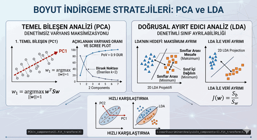
Principal Component Analysis (PCA) and Variance Maximization
PCA is an unsupervised algorithm. It does not need labels; its focal point is to represent the total variance (information) that the data possesses with the fewest possible components.
Mathematical Foundation and Eigenvectors
The operating logic of PCA relies on analyzing the covariance matrix ($S$) of the data to find the directions along which the data is most spread out (where variance is highest). These directions are called Principal Components.
PC1 (First Component): The direction that captures the greatest variance in the data.
PC2 (Second Component): The direction that is orthogonal to PC1 and maximizes the remaining variance.
This process is performed through eigenvalue and eigenvector calculation. The eigenvector corresponding to the largest eigenvalue of a covariance matrix $S$ determines the most dominant component of the data.
Determining the Number of Dimensions: Scree Plot and PoV
The Proportion of Variance (PoV) is used when deciding how many components to keep. If the first two components explain 90% of the total variance, reducing the data to these two dimensions keeps data loss minimal. In a Scree Plot, the “elbow” point is the most common method used to select the optimum number of components.
Class Separation with Linear Discriminant Analysis (LDA)
While PCA focuses on the data as a whole, LDA is a supervised approach. The fundamental goal of LDA is to maximize the separability between classes while reducing the data.
LDA’s Optimization Criterion
LDA optimizes two fundamental statistics:
Within-class scatter ($S_w$): Measures how close points belonging to the same class are to each other. It is desired for this to be minimum.
Between-class scatter ($S_b$): Measures how far the centers of different classes are from each other. It is desired for this to be maximum.
LDA creates a projection space that maximizes the ratio $J(w) = \frac{S_b}{S_w}$. In doing so, it provides a much more successful preprocessing step for classification models.
Comparative Analysis of PCA and LDA
Feature
PCA (Principal Component Analysis)
LDA (Linear Discriminant Analysis)
Learning Type
Unsupervised
Supervised
Goal
To preserve maximum variance
To maximize class separability
Input
Only features ($X$)
Features ($X$) and Labels ($y$)
Outliers
Sensitive (can bias the variance)
More resistant based on class centers
Use Case
Data compression, Denoising
Feature extraction before classification
Application and Technical Implementation with Python
In modern data science projects, these algorithms are generally implemented with the scikit-learn library. Below is a comprehensive code example regarding how to run both methods on a dataset.
import numpy as np
import matplotlib.pyplot as plt
from sklearn import datasets
from sklearn.decomposition import PCA
from sklearn.discriminant_analysis import LinearDiscriminantAnalysis
from sklearn.preprocessing import StandardScaler
# 1. Preparation of the Dataset (Iris dataset)iris = datasets.load_iris()
X = iris.data
y = iris.target
target_names = iris.target_names
# Standardization of data is important for PCA and LDAsc = StandardScaler()
X_scaled = sc.fit_transform(X)
# 2. PCA Implementation# We provide visualization by reducing to 2 componentspca = PCA(n_components=2)
X_pca = pca.fit_transform(X_scaled)
# 3. LDA Implementation# Since LDA is supervised, it also takes y labelslda = LinearDiscriminantAnalysis(n_components=2)
X_lda = lda.fit(X_scaled, y).transform(X_scaled)
# 4. Visualization of Resultsplt.figure(figsize=(12, 5))
# PCA Plotplt.subplot(1, 2, 1)
for color, i, target_name in zip(['navy', 'turquoise', 'darkorange'], [0, 1, 2], target_names):
plt.scatter(X_pca[y == i, 0], X_pca[y == i, 1], color=color, alpha=.8, lw=2, label=target_name)
plt.legend(loc='best', shadow=False, scatterpoints=1)
plt.title('PCA: Variance-Oriented Projection of Data')
# LDA Plotplt.subplot(1, 2, 2)
for color, i, target_name in zip(['navy', 'turquoise', 'darkorange'], [0, 1, 2], target_names):
plt.scatter(X_lda[y == i, 0], X_lda[y == i, 1], alpha=.8, color=color, label=target_name)
plt.legend(loc='best', shadow=False, scatterpoints=1)
plt.title('LDA: Class Separation-Oriented Projection')
plt.show()
# Printing Explained Variance Ratiosprint(f"PCA Explained Variance Ratio (PC1 + PC2): {np.sum(pca.explained_variance_ratio_):.2f}")
Advanced Notes and Technical Warnings
Necessity of Standardization
Since PCA looks at the variance of the data, data in different units (e.g., millimeters and kilometers) can mislead the algorithm. Just because the numerical values of a feature are very large does not mean it is more important. That is why it is critical to transform the data using methods like StandardScaler so that the mean is 0 and the standard deviation is 1.
Moving Beyond Linearity with Kernel Techniques
PCA and LDA are linear transformations. However, if the data has a circular or complex manifold structure, linear methods are insufficient. In this case, Kernel PCA is used to transport the data to a high-dimensional space (Hilbert space) where it is linearly separated.
Memory Management and Big Data
In very large datasets (Big Data), it may not be possible to load the entire covariance matrix into memory. In such cases, Incremental PCA (IPCA) is preferred, and the data is processed in small pieces (mini-batches).
Algorithmic Selection Strategy
Which method you choose depends entirely on the nature of your data and your ultimate goal. If your goal is only to compress the data and reduce noise, PCA, which does not use labels and preserves the general structure, is the safest harbor. However, if you have a labeled dataset and want to increase the performance of a classification model (like SVM, Random Forest), LDA, which clarifies the boundaries between classes, will yield much more effective results.
Dimensionality reduction is an inseparable part of modern machine learning pipelines. When applied correctly, it not only increases model speed but also allows us to build more robust and stable artificial intelligence systems by revealing the hidden patterns underlying the data.