We use cookies and other tracking technologies to improve your browsing experience on our website, to show you personalized content and targeted ads, to analyze our website traffic, and to understand where our visitors are coming from.
⚠️
GDPR & Cookie Policy Notice
In accordance with data protection regulations; the use of mandatory cookies is required for the core functions of our website to operate, ensure data security, and perform analytics. If you reject the use of cookies, it is not possible to benefit from the services on our website due to technical limitations and data synchronization interruptions. You must consent to the use of cookies to access the content on our site.
Delicate Balances and Strategic Approaches in Modern Machine Learning
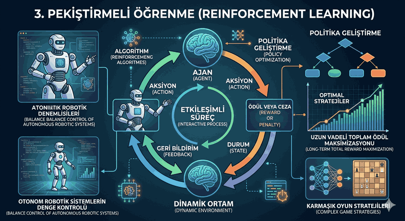
The artificial intelligence ecosystem is built upon two massive pillars in the processes of extracting meaning from data and transforming that meaning into action: supervised learning algorithms that draw geometric boundaries, and reinforcement learning models that act as experience-oriented decision-making mechanisms. In today’s complex datasets, making accurate predictions is not enough; it is vital to show resistance against noise and to develop the best strategy in dynamic environments.
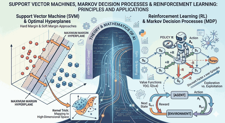
Figure 1: Delicate Balances and Strategic Approaches in Modern Machine Learning.
Support Vector Machines and Maximum Margin Optimization
Support Vector Machine (SVM) fundamentally reduces a classification problem to the problem of finding the optimal hyperplane in a high-dimensional space. However, the fundamental difference that distinguishes SVM from an ordinary logistic regression is the “maximum margin” principle.
Hyperplane and Geometric Robustness
An infinite number of lines (or hyperplanes) can be drawn that separate a dataset into two classes. However, most of these lines are prone to misclassification when faced with a noisy data point. SVM selects the hyperplane that keeps the gap (buffer zone) between classes the widest. This width is mathematically expressed by the formula $2/\|w\|$. Here, $\|w\|$ is the norm of the normal vector of the plane. Maximizing the margin is equivalent to minimizing the value $\|w\|^2/2$, and this is a quadratic programming problem.
Hard Margin and Soft Margin Distinction
If our dataset is perfectly linearly separable, Hard Margin SVM is used. There is no tolerance for error here:
$$y_i(w \cdot x_i + b) \geq 1$$
However, real-world data is noisy, and sometimes classes overlap. In this case, Soft Margin comes into play. By adding slack variables called $\xi$, some points are allowed to violate the margin in exchange for a certain penalty ($C$ parameter). The $C$ parameter is a critical hyperparameter that balances margin width with training error.
Kernel Trick: Leap from Low Dimension to High Dimension
When data is not linearly separable (e.g., a circular distribution), it is necessary to move the data to a higher dimension. However, calculating coordinates in high dimension is costly. The Kernel Trick allows us to calculate the interaction in high dimension using the inner products of points in low dimension without actually moving the data.
import numpy as np
from sklearn import svm
from sklearn.preprocessing import StandardScaler
from sklearn.model_selection import train_test_split
# Data Preparation and Scaling# SVM is very sensitive to scale differences, so StandardScaler is essential.scaler = StandardScaler()
X_scaled = scaler.fit_transform(X)
# Model Building (with RBF Kernel and C Parameter)clf = svm.SVC(kernel='rbf', C=1.0, gamma='scale')
clf.fit(X_train, y_train)
# Accessing Support Vectorssupport_vectors = clf.support_vectors_
print(f"Number of Support Vectors: {len(support_vectors)}")
Reinforcement Learning and Decision Making Mechanisms
Reinforcement Learning (RL) is a learning paradigm where an agent performs actions within an environment to maximize rewards. Unlike supervised learning, the agent is not told what to do; the agent discovers which action brings more reward by trial and error.
Agent and Environment Interaction
The process begins with the agent observing the current state ($S_t$). The agent chooses an action ($A_t$), and the environment returns the next state ($S_{t+1}$) and a reward ($R_{t+1}$) in response. This cycle continues until the agent develops a policy ($\pi$) that maximizes cumulative reward.
Episodic and Continuing Tasks
Episodic Tasks: There is a start and end point (e.g., a chess match). The total return is the sum of the steps.
Continuing Tasks: There is no natural end (e.g., energy management of a factory). Here, the discount factor ($\gamma$) is used for the convergence of the infinite sum:
If $\gamma = 0$, the agent is myopic (looks only at immediate reward); if $\gamma \to 1$, the agent thinks strategically and long-term.
Markov Decision Processes: The Mathematical Skeleton of RL
Most RL problems are modeled within the framework of Markov Decision Processes (MDP). A process having the “Markov” property means that the future depends only on the present moment, and the past is irrelevant.
MDP Components
State Set ($S$): All positions where the agent can be.
Action Set ($A$): Moves that can be made.
Transition Probability ($P$): Expressed by the formula $P(s' | s, a)$; it is the probability of transitioning to state $s'$ when action $a$ is taken in state $s$.
Reward Function ($R$): The numerical value determining the quality of the action taken.
Value Functions and Bellman Equations
The State-Value Function ($V(s)$) is used to understand how “good” a state is, and the Action-Value Function ($Q(s, a)$) is used to understand how good it is to take a specific action in a state. Optimal value functions are solved recursively via Bellman equations.
Exploration vs. Exploitation Trade-off
This is the biggest paradox of RL. Should the agent follow the best path it knows (exploitation), or should it try new paths to see if there is a better way (exploration)?
The most common solution is the $\epsilon$-greedy approach:
With a small probability ($\epsilon$), a random action is chosen (Exploration).
With the remaining large probability ($1-\epsilon$), the current best action is chosen (Exploitation).
A Simple Q-Learning Structure
import numpy as np
# Initialize Q-table (in State x Action dimensions)q_table = np.zeros([state_space_size, action_space_size])
# Hyperparameterslearning_rate =0.1discount_factor =0.95epsilon =0.1for episode in range(1000):
state = env.reset()
done =Falsewhilenot done:
# Action selection with Epsilon-greedyif np.random.uniform(0, 1) < epsilon:
action = env.action_space.sample()
else:
action = np.argmax(q_table[state])
next_state, reward, done, _ = env.step(action)
# Q-Value Update (Based on Bellman Equation) old_value = q_table[state, action]
next_max = np.max(q_table[next_state])
new_value = (1- learning_rate) * old_value + learning_rate * (reward + discount_factor * next_max)
q_table[state, action] = new_value
state = next_state
Key Differences and Use Cases Between SVM and RL
Although both technologies are part of artificial intelligence, their application areas and logic are polar opposites:
Feature
Support Vector Machines (SVM)
Reinforcement Learning (RL)
Learning Type
Supervised
Interactive
Data Requirement
Labeled datasets
Live interaction with environment
Fundamental Goal
Separate data with a hyperplane
Maximize cumulative reward
Decision Structure
Static (One-time prediction)
Dynamic (Sequential decisions)
Sensitivity
Highly sensitive to feature scaling
Sensitive to exploration/exploitation balance
Final Notes and Technical Recommendations
Success in data science comes from mastering the internal mechanisms of an algorithm rather than just choosing the right one. When using SVM, data normalization and choosing the right kernel determine the model’s noise resistance. On the RL side, the design of the reward function (reward shaping) determines whether the agent will “cheat” or truly learn the goal.
Especially in high-dimensional and noisy data, solving SVM via the Dual Form reduces computational cost by utilizing the kernel trick advantage. In RL projects, preferring modern architectures such as Deep Q-Networks (DQN), which is the combination of deep learning and RL, to manage complex state spaces will increase the agent’s generalization ability.