We use cookies and other tracking technologies to improve your browsing experience on our website, to show you personalized content and targeted ads, to analyze our website traffic, and to understand where our visitors are coming from.
⚠️
GDPR & Cookie Policy Notice
In accordance with data protection regulations; the use of mandatory cookies is required for the core functions of our website to operate, ensure data security, and perform analytics. If you reject the use of cookies, it is not possible to benefit from the services on our website due to technical limitations and data synchronization interruptions. You must consent to the use of cookies to access the content on our site.
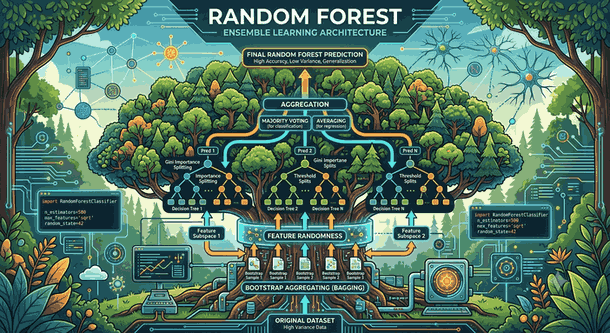
Technical Architecture and Implementation Principles of the Random Forest Algorithm
Within the “Ensemble Learning” framework of machine learning literature, Random Forest is a “supervised learning” algorithm that demonstrates high “generalization” capacity in both “classification” and “regression” tasks. The algorithm basically builds a forest of “Decision Trees.” However, this forest is not just a collection of ordinary trees; it is a statistically low-correlation structure where each tree is trained on different subsets of data and different “feature” groups.
Figure 1: Technical Architecture and Implementation Principles of the Random Forest Algorithm.
Transition from Decision Tree Structure to Ensemble Architecture
A single “Decision Tree” is quite vulnerable to variance in the dataset; that is, small changes in the training data can lead to dramatic fractures in the model’s structure. Random Forest minimizes this “high variance” problem with two fundamental statistical methods:
Bootstrap Aggregating (Bagging): Different “subsets” are created by taking samples with replacement from the training dataset. This allows the model to gain a “robust” structure by being trained on different data.
Feature Randomness (Feature Subspace): The “splitting” process to be performed at each “node” of each tree is done not over all “features,” but over a randomly selected “subspace.” This reduces the “correlation” between trees and increases the forest’s total predictive power.
Mathematical Framework and Variance Reduction
The power of the Random Forest algorithm is fixed by statistical laws. If we have $N$ number of “Decision Trees” and each has a variance of $\sigma^2$, the theoretical variance when these trees are averaged is:
Here, $\rho$ is the “correlation coefficient” between the trees. Random Forest minimizes the total variance by reducing the $\rho$ value through “feature randomness.” As the number of “estimators” ($N$) increases, the variance decreases, but after a point, due to the law of “diminishing returns,” the computational cost exceeds the performance gain.
Technical Application and Implementation with Python
In modern “data science” processes, the scikit-learn library offers this algorithm with high performance through the RandomForestClassifier and RandomForestRegressor classes. The code block below demonstrates the structuring of the model on a high-dimensional dataset and the basis of the “hyperparameter tuning” process.
import numpy as np
from sklearn.ensemble import RandomForestClassifier
from sklearn.model_selection import train_test_split
# Preparation of training data# n_estimators: Number of trees in the forest# criterion: 'gini' or 'entropy' (information gain criterion)# max_features: Maximum number of features to be evaluated at each noderf_model = RandomForestClassifier(
n_estimators=500,
criterion='gini',
max_depth=None,
min_samples_split=2,
min_samples_leaf=1,
max_features='sqrt',
bootstrap=True,
n_jobs=-1, # Parallel processor usage random_state=42)
# Training the modelrf_model.fit(X_train, y_train)
# Prediction performance of the modelaccuracy = rf_model.score(X_test, y_test)
print(f"Model Accuracy: {accuracy:.4f}")
Hyperparameter Optimization and Model Dynamics
The success of the Random Forest algorithm depends on the correct configuration of “hyperparameter” values. The most critical settings are as follows:
n_estimators: The number of trees. It is generally chosen between 100 and 1000. More trees increase “training” time linearly but improve the “stability” rate of the model.
max_features: The number of “features” selected to split a “node.” It is recommended to start with $\sqrt{\text{total\_features}}$ for “classification” and generally $\text{total\_features}/3$ for “regression.”
min_samples_leaf: The minimum number of samples that must be in the leaves. Increasing this value prevents the model from focusing on details (“noise”), thereby reducing the risk of “overfitting” (regularization effect).
Feature Importance
One area where Random Forest provides “white-box” like transparency is the degree of importance of variables. The algorithm calculates how effective each “feature” value is on the target variable by summing the “Gini impurity” drops at the nodes of each tree.
import pandas as pd
import matplotlib.pyplot as plt
# Extracting importance degreesimportances = rf_model.feature_importances_
indices = np.argsort(importances)[::-1]
# Visualizationplt.figure(figsize=(10, 6))
plt.title("Feature Importances")
plt.bar(range(X_train.shape[1]), importances[indices])
plt.show()
Operational Advantages and Limitations
The Random Forest algorithm owes the reasons it is widely preferred at an industrial scale to its low “preprocessing” requirement.
Important Note: Random Forest does not require a “scaling” (Normalization/Standardization) process for data. This is because “Decision Tree” structures fundamentally make decisions based on “threshold” values according to “if-else” logic; the distribution of the data does not directly affect this logic.
Feature
Technical Impact
Outlier Resilience
Since it is tree-based, it is minimally affected by extreme values.
Non-linearity
It successfully captures non-linear relationships in data with “node” splits.
Memory Complexity
A large number of trees can lead to high RAM consumption.
Inference Latency
A large number of trees can cause slowness in the “inference” stage.
Conclusion
Random Forest successfully establishes the balance between “bias” and “variance” thanks to the “Bagging” strategy. However, today, “Gradient Boosting”-based algorithms such as XGBoost, LightGBM, and CatBoost have pushed the performance limits of Random Forest further. Nevertheless, the model’s level of “interpretability” and high tolerance for “noisy data” make it an indispensable “baseline” model in “data science pipeline” structures.