We use cookies and other tracking technologies to improve your browsing experience on our website, to show you personalized content and targeted ads, to analyze our website traffic, and to understand where our visitors are coming from.
⚠️
GDPR & Cookie Policy Notice
In accordance with data protection regulations; the use of mandatory cookies is required for the core functions of our website to operate, ensure data security, and perform analytics. If you reject the use of cookies, it is not possible to benefit from the services on our website due to technical limitations and data synchronization interruptions. You must consent to the use of cookies to access the content on our site.
Reduction Methods and Numerical Analysis Approaches in Linear Circuit Analysis
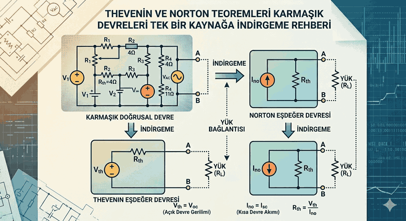
Electrical circuits, especially in modern microelectronics and power systems, form massive networks by combining thousands of passive and active components. Attempting to solve the voltage and current values at every point in these networks using classical Kirchhoff’s laws means dealing with massive systems of linear equations. At this point, Thevenin and Norton Theorems, which reduce the rest of the circuit to a single voltage or current source, become a cornerstone of the engineering discipline.
Figure 1: Reduction Methods and Numerical Analysis Approaches in Linear Circuit Analysis.
1. Basic Theoretical Framework and Equivalence Principle
A linear circuit, no matter how complex the independent sources and resistors within it are, behaves like a two-terminal (port) box when viewed from the outside. Thevenin and Norton theorems allow us to define the electrical characteristics of this “black box” with only two parameters.
Thevenin Theorem: Voltage-Oriented Approach
Thevenin’s theorem argues that the interaction between any two terminals of a linear circuit can be represented by a voltage source ($V_{th}$) and an internal resistance ($R_{th}$) connected in series to these terminals. Here, $V_{th}$ is the voltage measured when the terminals are open-circuited; $R_{th}$ is the equivalent resistance seen from the terminals when all independent sources are “killed” (voltage sources short-circuited, current sources open-circuited).
Figure 2: Thevenin Theorem.
Norton Theorem: Current-Oriented Approach
The Norton theorem is the dual of Thevenin. It is based on modeling the circuit as a current source ($I_{no}$) and a resistance ($R_{no}$) connected in parallel to it. The Norton current is the current flowing when the relevant terminals of the circuit are short-circuited. Interestingly, the equivalent resistance value used in both theorems is equal to each other ($R_{th} = R_{no}$).
2. Analytical Calculation Algorithms
The mathematical steps followed when reducing a circuit must follow a systematic order to minimize the margin of error.
Step 1: Open Circuit Voltage and Short Circuit Current
The load resistor to be analyzed is disconnected from the circuit. The potential difference at the resulting open terminals is determined as $V_{oc} = V_{th}$. Then, these terminals are connected with an ideal conductor to calculate the flowing $I_{sc} = I_{no}$ current.
Step 2: Determination of Equivalent Resistance
If there are only independent sources in the circuit, resistor combinations can be calculated directly by deactivating the sources. However, if there are dependent sources (VCVS, CCVS, etc.) in the circuit, it is mandatory to apply a test source ($V_{test}$) to the terminals. In this case:
$$R_{th} = \frac{V_{test}}{I_{test}}$$
the result is reached through this equation.
Important Note: According to the Maximum Power Transfer Theorem, for the power transferred to the load to be maximized, the load resistance ($R_L$) must be equal to the Thevenin equivalent resistance ($R_{th}$). This is critical, especially in RF circuits requiring impedance matching.
3. Numerical Analysis and Computational Techniques
Today, solving complex circuits by hand is practically impossible. At this point, the power of circuit simulation software (SPICE, LTspice) and numerical calculation libraries (NumPy, SciPy) is utilized.
Solving Circuit Matrices with Python
Nodal Analysis is used to find the Thevenin equivalent of a circuit. The following code block forms a basis for calculating the potential difference between specific nodes and thus the Thevenin parameters by using the coefficient matrix of a circuit.
import numpy as np
defcalculate_thevenin(conductance_matrix, current_vector, node_a, node_b):
"""
Calculates the Thevenin equivalent using the node matrices of a linear circuit.
Solves the system of equations G * V = I.
"""try:
# Calculate node voltages voltages = np.linalg.solve(conductance_matrix, current_vector)
# Open circuit voltage (V_th) v_th = voltages[node_a] - voltages[node_b]
# For equivalent resistance (R_th) calculation:# Extracted from the inverse of the matrix with passive sources. resistance_matrix = np.linalg.inv(conductance_matrix)
r_th = resistance_matrix[node_a, node_a] + \
resistance_matrix[node_b, node_b] - \
2* resistance_matrix[node_a, node_b]
return v_th, r_th
except np.linalg.LinAlgError:
returnNone, "Matrix is singular, no solution."# Example Usage:# Conductance matrix of a 3-node circuit (in Siemens)G = np.array([[0.5, -0.2, 0],
[-0.2, 0.7, -0.1],
[0, -0.1, 0.3]])
# Source current vector (Amperes)I = np.array([2, 0, 1])
v_th, r_th = calculate_thevenin(G, I, 0, 2)
print(f"Thevenin Voltage: {v_th:.2f} V")
print(f"Thevenin Resistance: {r_th:.2f} Ohm")
print(f"Norton Current: {(v_th/r_th):.2f} A")
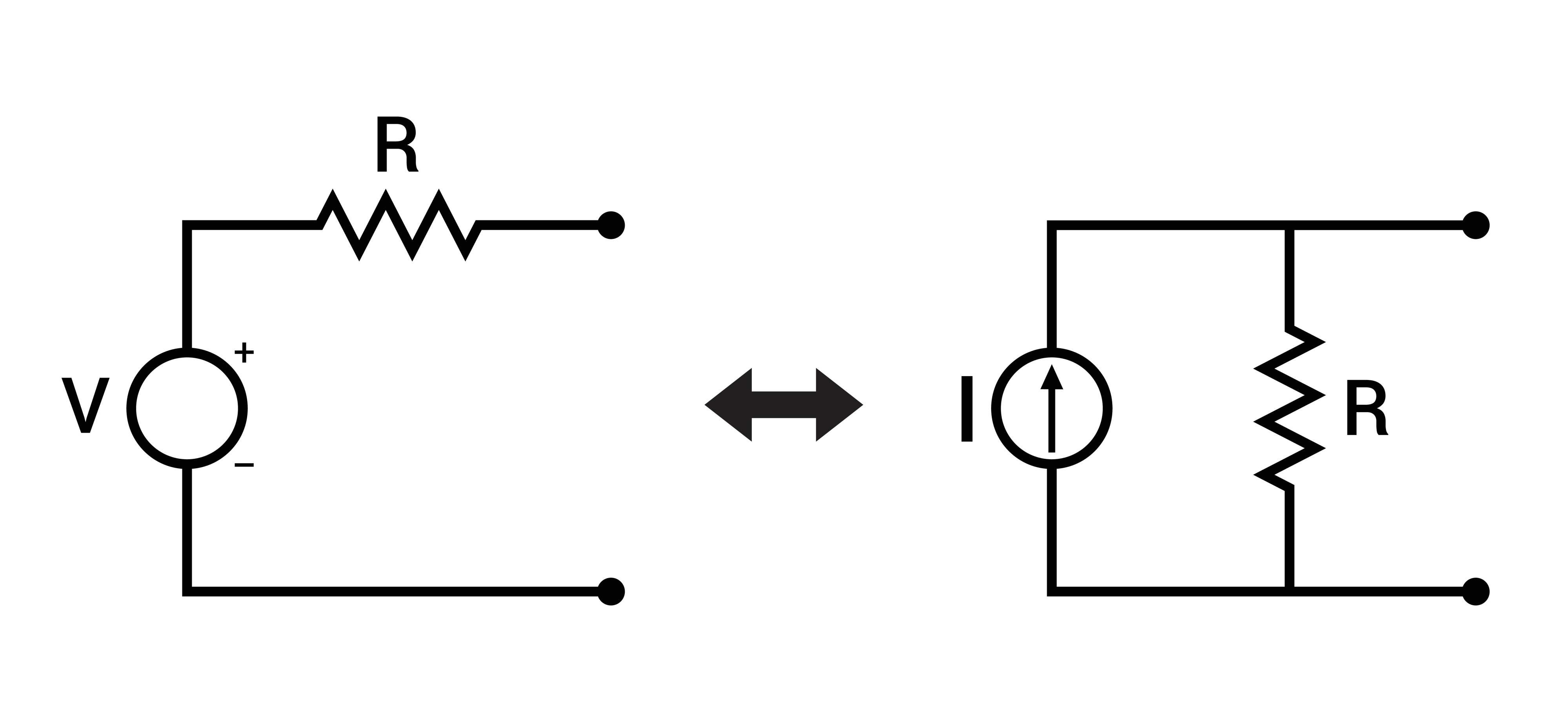
4. Source Transformation and Duality Relationship
Switching between Thevenin and Norton models increases flexibility in circuit analysis. This transition is based on the Ohm’s law principle:
$V_{th} = I_{no} \times R_{th}$
$I_{no} = \frac{V_{th}}{R_{th}}$
This transformation is of vital importance, especially in cascading reduction (Source Transformation) of circuits with many branches. By converting a voltage source into a current source, we can obtain parallel branches, thus simplifying the circuit algebraically more quickly.
5. Application Areas and Engineering Practices
Thevenin and Norton theorems are not just academic exercises; they are the basis of industrial standards:
Power Systems: The behavior of a city grid at a single transformer output is modeled with a Thevenin equivalent to perform short-circuit analyses.
Instrumentation: Used to determine the output impedances of sensors and calculate the loading effect of the measuring device (voltmeter/oscilloscope) on the circuit.
Integrated Circuit Design (IC): The interface interactions of processor blocks consisting of billions of transistors are simulated via these simplified models.
6. Technical Analysis and Performance Comparison
Which method is more efficient when reducing a complex circuit depends on the topology of the circuit. If the circuit consists mainly of series branches, Thevenin, and if there are dense parallel current branches, the Norton method will reduce the processing load.
Comparative Notes:
Thevenin: As it approaches the $R_{th}=0$ condition with the ideal voltage source assumption, the system “stiffens”. It is ideal for modeling low internal resistance power supplies.
Norton: It provides more consistent results in the analysis of high internal resistance systems (e.g., photovoltaic cells or transistor collector outputs).
Sensitivity: In numerical analysis, the approach of resistance values to zero can cause the matrices to become unstable (ill-conditioned). In these cases, using the Norton approach via conductance (G) matrices increases numerical stability.
7. Conclusion and Future Perspective
Thevenin and Norton theorems have formed the main backbone of electrical engineering since the 19th century. Today, even artificial intelligence and machine learning-based circuit design tools use these basic reduction algorithms in their optimization processes. A engineer’s or programmer’s ability to reduce a complex structure to its simplest components is the only way to predict the behavior of the system.
With the development of numerical methods and software libraries, these theorems no longer exist only on paper but as dynamic models running within real-time control systems. Especially in renewable energy systems, this “reduction discipline” will maintain its indispensability for modeling grid interaction.