We use cookies and other tracking technologies to improve your browsing experience on our website, to show you personalized content and targeted ads, to analyze our website traffic, and to understand where our visitors are coming from.
⚠️
GDPR & Cookie Policy Notice
In accordance with data protection regulations; the use of mandatory cookies is required for the core functions of our website to operate, ensure data security, and perform analytics. If you reject the use of cookies, it is not possible to benefit from the services on our website due to technical limitations and data synchronization interruptions. You must consent to the use of cookies to access the content on our site.
Mathematical Architecture of Complex Circuits and Nodal Analysis Method
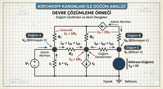
The analysis of electrical circuits is an interdisciplinary process where fundamental physical laws are blended with linear algebra. In modern engineering applications, especially in integrated circuit design and power systems simulation, it is necessary to adopt a systematic approach rather than examining the circuit on a component-by-component basis. At this point, Nodal Analysis, built upon Kirchhoff’s Current Law (KCL), allows us to reach the solution set by reducing unknown voltages in the circuit to a systematic matrix form.
Figure 1: Mathematical Architecture of Complex Circuits and Nodal Analysis Method.
Kirchhoff’s Laws and Theoretical Foundation
Kirchhoff’s Current Law, which lies at the heart of nodal analysis, is based on the principle of conservation of charge. The algebraic sum of currents entering a closed node must be equal to the sum of currents leaving that node. Expressed mathematically:
$$\sum_{k=1}^{n} I_k = 0$$
This equation allows for the generation of an independent linear equation for each node in the circuit. In nodal analysis, the primary goal is to determine the potential differences of all nodes relative to a reference (chassis/ground) point on the circuit.
Selection and Importance of the Reference Node
Before beginning the analysis, the potential of one point in the circuit is assumed to be $0V$. Usually, the point where the most components are connected or where the negative terminals of voltage sources meet is selected as the “reference node.” This choice reduces the number of unknowns in the system of equations by one, thereby easing the computational burden.
Nodal Analysis Implementation Steps
A systematic solution process minimizes the margin of error. Using an engineering approach, we can break this process down into the following steps:
Identification of Nodes: All points where more than two components meet (essential nodes) are marked.
Assignment of Reference Node: One point is designated as ground ($V_g = 0$).
Writing KCL Equations: Kirchhoff’s Current Law is applied to each $n$ node other than the reference. Currents are expressed in terms of node voltages using Ohm’s Law ($I = V/R$).
Matrix Formulation: The resulting linear equations are converted into the form $[G][V] = [I]$. Here, $[G]$ represents the conductance matrix, $[V]$ represents the node voltages, and $[I]$ represents the current sources.
Numerical Solution: Unknown voltages are found using methods such as Cramer’s rule, Gaussian elimination, or LU decomposition.
The Concept of a Supernode
If there is only an independent or dependent voltage source between two nodes and this source is not connected to the reference node, the “Supernode” technique is applied. In this case, the two nodes are treated as a single surface, and the KCL equation is written for the entire surface. Additionally, a “constraint equation” defining the source voltage is included in the system.
Practical Circuit Example and Analytical Solution
Let us consider a circuit with three basic nodes and two different current sources. Let our resistance values be $R_1, R_2, R_3$ and our node voltages be $V_1, V_2$.
When these equations are arranged, the variables take on a matrix structure. Modern circuit simulators (SPICE, etc.) generate results by solving these exact conductance matrices in the background.
Software Approach: Automated Solution with Python and NumPy
Nowadays, it is impossible to solve large-scale circuits by hand. Engineering tools treat circuit topology as a matrix. Below, a professional approach is presented on how a circuit matrix can be solved using the NumPy library.
import numpy as np
defsolve_nodal_analysis(conductance_matrix, current_vector):
"""
Solves node voltage equations in the form [G][V] = [I].
G: Conductance matrix (Siemens)
I: Node current vector (Amperes)
"""try:
# Instead of inverting the matrix, we use the more stable solve method node_voltages = np.linalg.solve(conductance_matrix, current_vector)
return node_voltages
except np.linalg.LinAlgError:
return"Matrix is singular. Check circuit topology."# Example Circuit Parameters# Let R1=10, R2=5, R3=20 ohms. Conductance G = 1/Rg1, g2, g3 =1/10, 1/5, 1/20# Node 1 equation: (g1 + g2)V1 - g2V2 = I1# Node 2 equation: -g2V1 + (g2 + g3)V2 = I2G = np.array([
[(g1 + g2), -g2],
[-g2, (g2 + g3)]
])
I = np.array([2, -1]) # Net currents entering nodes (Amperes)voltages = solve_nodal_analysis(G, I)
print("--- Circuit Analysis Results ---")
for i, v in enumerate(voltages):
print(f"Node V{i+1} Voltage: {v:.4f} Volts")
Technical Analysis of the Code
The algorithm above is the direct equivalent of linear algebra in electrical theory. The np.linalg.solve function uses low-level LAPACK routines to solve systems in the form $Ax = B$. This maximizes performance, especially in the analysis of high-density circuits (LSI) with thousands of nodes.
Advanced Circuit Analysis Libraries
If you require not just simple matrix solutions, but also frequency response (AC Analysis) or transient analysis, more specific libraries in the Python ecosystem come into play:
PySpice: Provides full access to the Berkeley SPICE simulator via Python. It is an industry standard when working with realistic circuit elements (transistors, diodes).
SciPy (Signal Module): Ideal for analyzing the transfer functions ($H(s)$) of circuits and plotting Bode diagrams.
Conductance Instead of Resistance: When performing nodal analysis, using conductance ($G = 1/R$) values instead of resistance ($R$) values simplifies addition operations during matrix setup and reduces calculation errors.
Dependent Sources: If there is a dependent source (VCVS, CCVS, etc.) in the circuit, the control variables of these sources must be added to the system in terms of node voltages. This may break the symmetric structure of the matrix, but it does not change the solution method.
Sensitivity Analysis: The effect of parametric changes (e.g., the tolerance margin of a resistor) on the total voltage distribution should be examined by creating a Jacobian matrix with the help of partial derivatives.
Conclusion and Future Projection
Nodal analysis is not just a theoretical course topic; it is also the core of modern automation and simulation software. This deterministic approach offered by Kirchhoff’s Laws is even used in the hardware modeling of artificial neural networks (Neuromorphic Computing) along with the development of semiconductor technology. For engineers, the ability to integrate these methods with software tools is one of the most critical skills that accelerate design processes.
As the complexity of electronic systems increases, algorithmic solutions built upon these fundamental laws will remain the only way to ensure system stability. An efficient analysis process is born from the combination of accurate topological modeling and powerful computational tools.