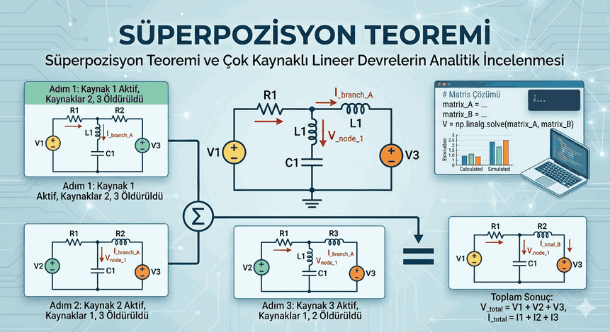
Superposition Theorem and Analytical Investigation of Multi-Source Linear Circuits

The Superposition Theorem, one of the cornerstones of electrical and electronics engineering, is a mathematical approach that reduces complex circuit networks into solvable parts. Especially in linear circuits containing multiple independent voltage or current sources, isolating the individual effect of each source on the system is of critical importance in design and analysis processes.

1. Theoretical Foundations of Linearity and Superposition

The Superposition Theorem is only valid in linear circuits. For a circuit to be considered linear, it must satisfy the properties of additivity and homogeneity. Mathematically, if $x$ is the input and $y$ is the output of a system, the equality $f(ax_1 + bx_2) = af(x_1) + bf(x_2)$ must hold.

In this context, passive components such as resistors, capacitors, and inductors are considered linear elements (under ideal conditions). However, in circuits containing non-linear elements such as diodes and transistors, this theorem cannot be applied directly; in this case, linearization must be performed using small-signal models.

Fundamental Principle

In a circuit with multiple independent sources, the current in any branch or the voltage between any two points is equal to the algebraic sum of the currents or voltages produced by each source acting alone (while other sources are killed).

2. Passivization (Killing) of Sources

The most critical step when applying the theorem is to neutralize all independent sources other than the one being analyzed. During this process, the topological structure of the circuit must be preserved, and only the internal resistances of the sources should be considered:

• Voltage Sources: The internal resistance of an ideal voltage source is zero. Therefore, it is short-circuited when passivized.
• Current Sources: The internal resistance of an ideal current source is infinite. Therefore, it is open-circuited when passivized.
• Dependent Sources: Since these sources depend on a variable at another point in the circuit, they are never killed. They must remain active throughout the analysis.

3. Application Steps and Methodology

For a systematic analysis, the following algorithm must be followed:

1. Source Selection: One of the independent sources in the circuit is selected.
2. Passivizing Others: All independent voltage sources other than the selected one are short-circuited, and current sources are open-circuited.
3. Partial Analysis: The circuit is solved for the single selected source using standard methods (Ohm’s Law, Kirchhoff’s Laws, Nodal/Mesh Analysis). The current ($i_1, i_2, ...$) or voltage ($v_1, v_2, ...$) values in the relevant branch are recorded, paying attention to their directions.
4. Repetition: This process is repeated separately for each independent source in the circuit.
5. Algebraic Sum: All partial results obtained are summed according to the reference directions determined at the beginning.

Important Note: Power ($P = I^2 \cdot R$ or $P = V^2 / R$) is not a linear function. For this reason, superposition cannot be applied directly in power calculations. If the total power is to be found, the total current or total voltage must be found first, and then the power formula should be applied.

4. Programming and Numerical Simulation Approaches

In modern engineering, these calculations are validated through software as well as being done by hand. Especially for solving large-scale circuit matrices, languages like Python and MATLAB are widely used.

Circuit Analysis with Python: Using SciPy and NumPy

The following code example is an approach that solves nodal voltages in a circuit consisting of two voltage sources and resistors using the matrix method (Nodal Analysis). To manually simulate superposition, we can reset the sources and run them in a loop.

import numpy as np

def solve_circuit(sources, resistances):
    """
    Nodal equations solution for a simple two-mesh circuit.
    sources: [V1, V2] voltage values
    resistances: [R1, R2, R3] resistance values
    """
    # G1, G2, G3 conductance values (1/R)
    G = [1/r for r in resistances]
    
    # Matrix Form: G * V = I
    # Assuming an example bridge circuit or parallel node structure
    matrix_A = np.array([
        [G[0] + G[2], -G[2]],
        [-G[2], G[1] + G[2]]
    ])
    
    matrix_B = np.array([sources[0] * G[0], sources[1] * G[1]])
    
    try:
        node_voltages = np.linalg.solve(matrix_A, matrix_B)
        return node_voltages
    except np.linalg.LinAlgError:
        return "Matrix is singular, no solution."

# Superposition Experiment
R = [100, 200, 150] # Ohm
V_total = [12, 5]    # Volt

# 1. Source active, 2. Source off (0V)
result_1 = solve_circuit([12, 0], R)
# 2. Source active, 1. Source off (0V)
result_2 = solve_circuit([0, 5], R)

# Total Result
total_result = result_1 + result_2

print(f"Partial Voltages (V1 active): {result_1}")
print(f"Partial Voltages (V2 active): {result_2}")
print(f"Total Nodal Voltages: {total_result}")

Software Libraries and Tools

• Spice (LTspice, PSpice): These industry-standard tools allow you to analyze superposition using the .step command or by resetting sources.
• PySpice: Ideal for creating and solving netlists of complex circuits using the Ngspice engine via Python.
• SciPy (Optimize & LinAlg): The fundamental library for matrix solutions and optimization operations.

5. Technical Details to Consider in Precision Calculations

The reason the superposition theorem is described as “precise” is that it provides the ability to model the error margin (tolerance) and temperature coefficient of each source separately.

Error Analysis and Tolerances

Production tolerances on resistors ($\pm \%1, \pm \%5$) play a critical role in high-precision medical or military devices. With the superposition method, it can be determined which source is more sensitive to tolerance changes (sensitivity analysis).

Frequency Domain Analysis (AC Circuits)

When applying superposition in AC circuits, the frequencies of the sources may differ. If there are sources with different frequencies, circuit impedances ($Z_L = j\omega L$, $Z_C = 1/j\omega C$) must be recalculated for each frequency. The results are summed in the time domain ($t$) to obtain complex waveforms.

6. Boundary Conditions and Disadvantages

Although it is a powerful tool, the Superposition Theorem is not the most efficient path in every scenario:

1. Computational Intensity: As the number of sources increases (e.g., a network with 10 sources), 10 separate circuit analyses must be performed. In this case, performing a single matrix solution using the Nodal Voltages or Mesh Currents method is much faster.
2. Dependent Source Complexity: There is a high probability of error in circuits with dependent sources, because these sources cannot be passivized and must be included in the equations for each partial analysis.
3. Power Calculation Fallacy: The most common engineering mistake is trying to reach the total power by summing partial powers. It must be remembered that $(a+b)^2 \neq a^2 + b^2$.

Conclusion

The Superposition Theorem is not just a calculation method in the analysis of linear systems, but also a perspective. It reduces the complexity of a system to simplicity with a “divide and conquer” strategy. In engineering practice, especially in fields like RF (Radio Frequency) design and signal processing, it is indispensable for understanding the effect of different signal components. When integrated with the software world, it forms the basis of powerful algorithms that can perform network optimization on large datasets.

In advanced circuit analysis, this theorem is combined with Thevenin and Norton theorems to produce much faster and error-free results using equivalent models of certain parts of the circuit. Not neglecting the internal resistances of sources in precision calculations and checking the mathematical consistency of each step are the keys to a professional analysis.